The ACE1 Electrical Impedance Tomography System for Thoracic Imaging

Abstract

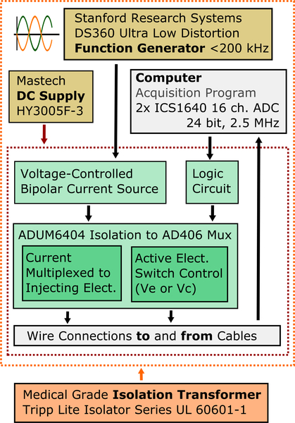
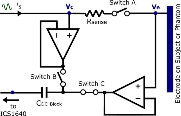
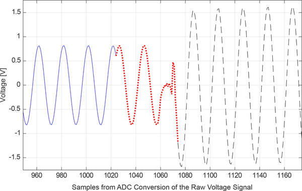
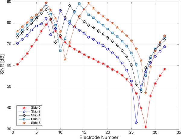
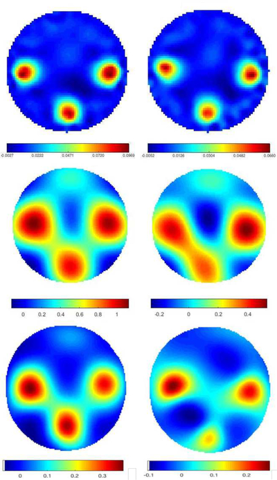
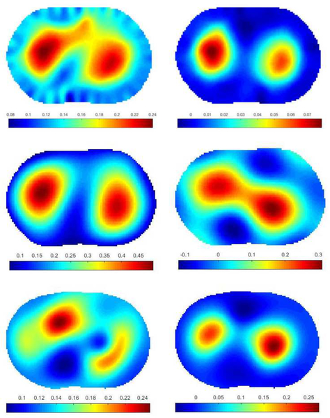
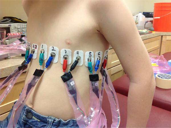
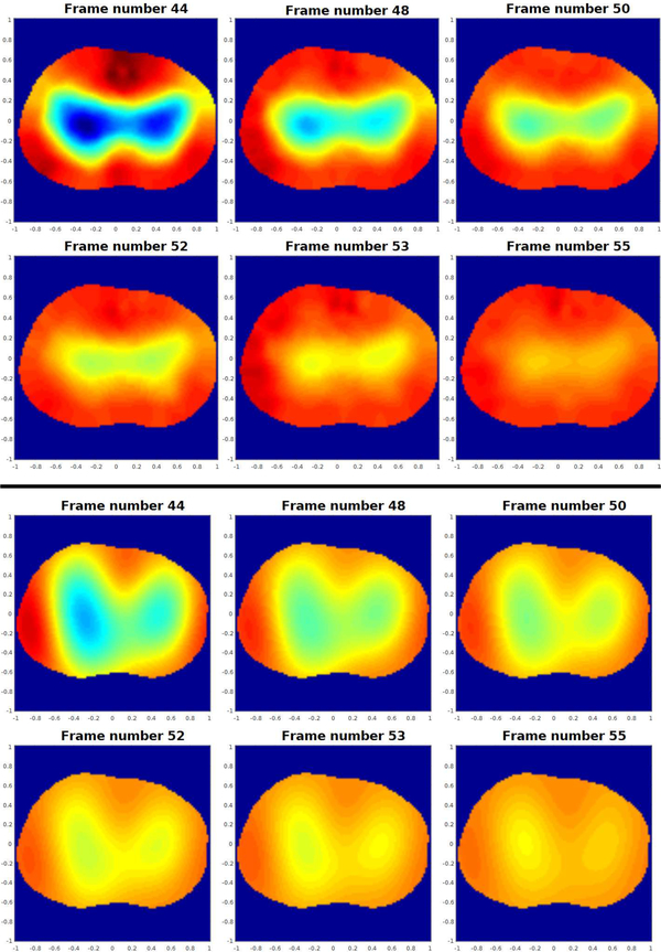
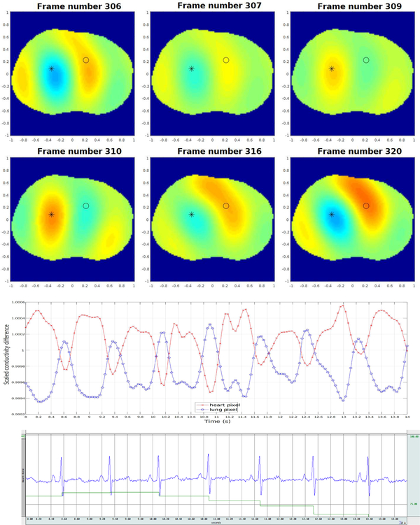
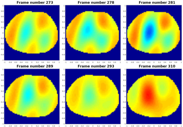
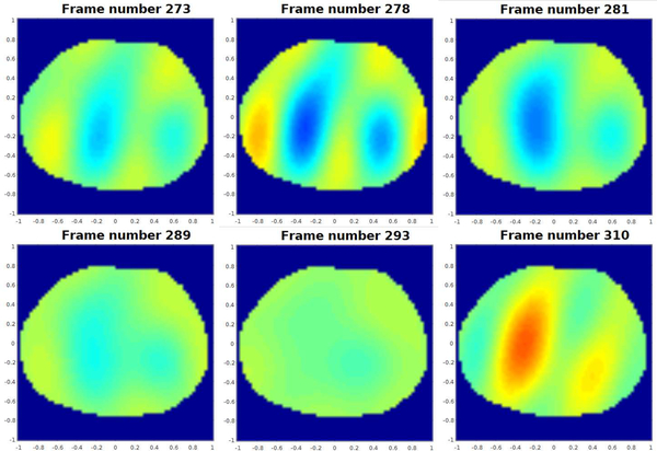
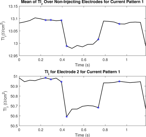
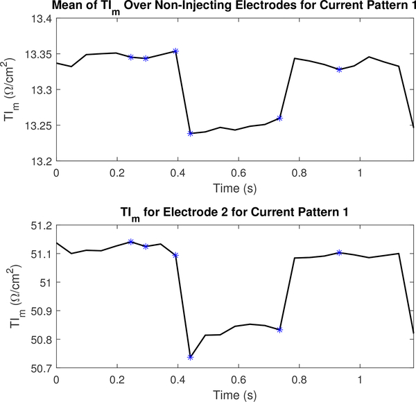
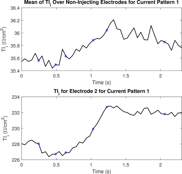
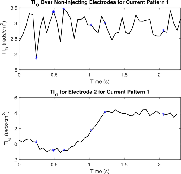
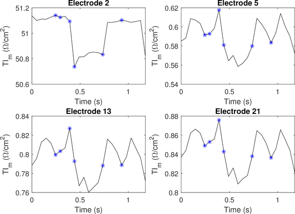
The design and performance of the ACE1 (Active Complex Electrode) electrical impedance tomography system for single-ended phasic voltage measurements is presented. The design of the hardware and calibration procedures allow for reconstruction of conductivity and permittivity images. Phase measurement is achieved with the ACE1 active electrode circuit which measures the amplitude and phase of the voltage and the applied current at the location at which current is injected into the body. An evaluation of the system performance under typical operating conditions includes details of demodulation and calibration and an in-depth look at insightful metrics, such as signal-to-noise ratio variations during a single current pattern. Static and dynamic images of conductivity and permittivity are presented from ACE1 data collected on tank phantoms and human subjects to illustrate the system's utility.

Keywords: biomedical imaging; electrical impedance tomography; thoracic imaging.

Fig. 1.

As shown in this overview of the ACE1 system design, it uses multiplexed digital signals to control current application and acquisition of voltages on the active electrodes (V_e or V_c).

Fig. 2.

The design of the ACE1 active electrode allows for determining injected current and measuring electrical potentials arising on the surface of the skin.

Fig. 3.

Samples located in the middle of the raw voltage signal of a single injecting channel can be used illustrate key components of ACE1 measurements. The 2048 samples in the raw voltage signal on a tank phantom was sampled at 2.5 MHz. The solid blue line is V_e. The dotted red line is $V_c^o$ and includes the discarded transient from the switching operation (1060–1070), and the dashed black line is $V_c^{cl}$.

Fig. 4.

Experimental signal-to-noise ratio differences were computed for each electrode for current pattern (k) 7 from 5 different datasets using different skip patterns. Each dataset contains 250 frames of data collected on a saline-filled tank at 16 frames/second. In k=7, electrode 7 is an injecting electrode and the skip pattern specifies the number of electrodes in between 7 and the next injecting electrode.

Fig. 5.

Test set-up where all of the ACE1 cables were connected to the same voltage source and 100 frames of data were collected. Inputs to the ACE1 current source were grounded.

Fig. 6.

Phase reproducibility at 125 kHz for 250 frames of tank data acquired at 1024 sample/rate for a single current pattern (k = 18).

Fig. 7.

Max voltage differences over all electrodes and current patterns for copper and plastic pipe targets in the center of a saline-filled tank compared to voltages in a homogeneous tank with data collected at 125 kHz with 1.8 mS/cm saline and current amplitude of 2.4 mA.

Fig. 8.

Photos of the cucumber targets in the saline-filled tank. Left: Triangle configuration of cucumber targets. Right: Watermelon “lungs” and agar “heart” in a saline bath.

Fig. 9.

Difference images of cucumber targets. Top row: computed with 5 iterations of the Gauss-Newton method. Center row: computed with Calderón’s method. Bottom row: computed with the D-bar method for complex conductivities. Left: conductivity σ, Right: susceptivity ωϵ. Units are in S/m.

Fig. 10.

Absolute images of melon and agar targets. Top row: computed with the Gauss-Newton method for complex admittivities. Center row: computed with Calderón’s method. Bottom row: computed with the the D-bar method for complex conductivities. Left: conductivity σ, Right: susceptivity ωϵ. Units are in S/m.

Fig. 11.

Data collection on a healthy eight-year old subject at CSU.

Fig. 12.

Sequence of conductivity difference images reconstructed from data collected during exhalation depicting changes due to ventilation in the human chest. Top set of images: computed with the Gauss-Newton method. Bottom set of images: computed with the D-bar method for real-valued conductivities. Here red corresponds to high conductivity and blue to low conductivity. The images are displayed in DICOM orientation.

Fig. 13.

Top: Sequence of conductivity difference images from the D-bar method for real-valued conductivities collected during breath-holding depicting changes due to perfusion in the human chest. Here red corresponds to high conductivity and blue to low conductivity. The images are displayed in DICOM orientation. Center: Time trace (in number of frames) of the reconstructed conductivity value in a pixel from the heart region (designated by a black * in the sequence of images above and plotted in the time trace in red), and the reconstructed conductivity value in a pixel from the lung region (designated by a black o in the sequence of images above and plotted in the time trace in blue). The rapid decrease in conductivity in the heart pixel is accompanied by a rapid increase in the lung pixel, corresponding to the contraction of the ventricles. Bottom: ECG data collected using Biopac simultaneously with the EIT data in this figure. The blue line is the output of the three-lead EKG and the green line is the average heart rate from the Biopac output.

Fig. 14.

Time snapshots of conductivity difference images in the ventilator sequence computed using Calderón’s method. Here red corresponds to high conductivity and blue to low conductivity. The images are displayed in DICOM orientation.

Fig. 15.

Time snapshots of susceptivity difference images in the ventilatory sequence computed using Calderón’s method. Here red corresponds to high susceptivity and blue to low susceptivity. The images are displayed in DICOM orientation.

Fig. 16.

The real component of the transfer impedance (TI_r) for non-injecting electrodes and the leading injecting electrode or l = 2 for the first current pattern (k =1). Each asterisk corresponds to the sequential series of images shown in Figure 13.

Fig. 17.

The magnitude component of the transfer impedance (TI_m) for non-injecting electrodes and the leading injecting electrode or l =2 for the first current pattern (k =1). Each asterisk corresponds to the sequential series of images shown in Figure 13.

Fig. 18.

The imaginary component of the transfer impedance (TI_i) for non-injecting electrodes and the leading injecting electrode or l =2 for the first current pattern (k =1). Each asterisk corresponds to the sequential series of images shown in Figure 15.

Fig. 19.

The phase component of the transfer impedance (TI_θ) for non-injecting electrodes and the leading injecting electrode or l =2 for the first current pattern (k =1). Each asterisk corresponds to the sequential series of images shown in Figure 15.

Fig. 20.

The magnitude component of the transfer impedance (TI_m) for injection electrode l =2, as well as 3 non-injecting electrodes. Each asterisk corresponds to the sequential series of images shown in Figure 15.

Fig. 21.

The phase component of the transfer impedance (TI_θ) for injection electrode l = 2, as well as 3 non-injecting electrodes. Each asterisk corresponds to the sequential series of images shown in Figure 15.

References

1. Holder D, Ed., Electrical impedance tomography; methods, history, and applications. IOP publishing Ltd., 2005.
1. Costa E, Lima R, and Amato M, “Electrical impedance tomography,” Current Opinion in Critical Care, vol. 15, pp. 18–24, 2009. - PubMed
1. Mueller J and Siltanen S, Linear and Nonlinear Inverse Problems with Practical Applications. SIAM, 2012.
1. Blankman P and Gommers D, “Lung monitoring at the bedside in mechanically ventilated patients,” Current Opinion in Critical Care, vol. 18, no. 3, pp. 261–266, 2012. - PubMed
1. Pham T, Yuill M, Dakin C, and Schibler A, “Regional ventilation distribution in the first 6 months of life,” European Respiratory Journal, vol. 37, no. 4, pp. 919–924, 2011. - PubMed
LinkOut - more resources