Auditory activity is diverse and widespread throughout the central brain of Drosophila

Abstract

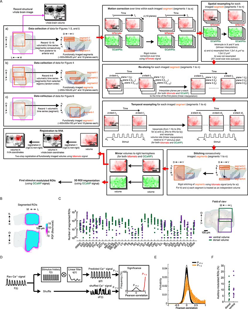
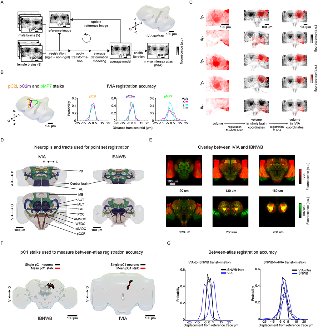
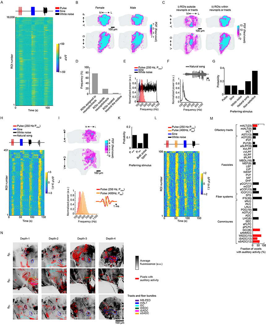
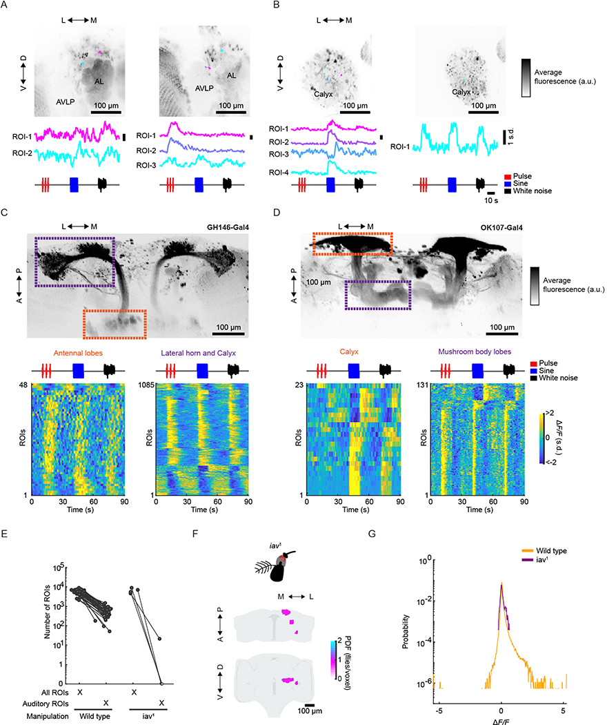
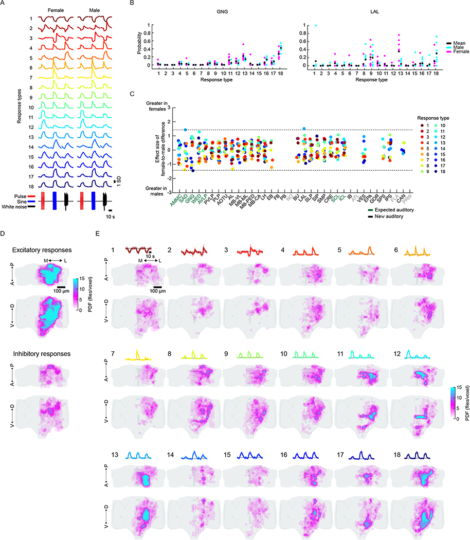
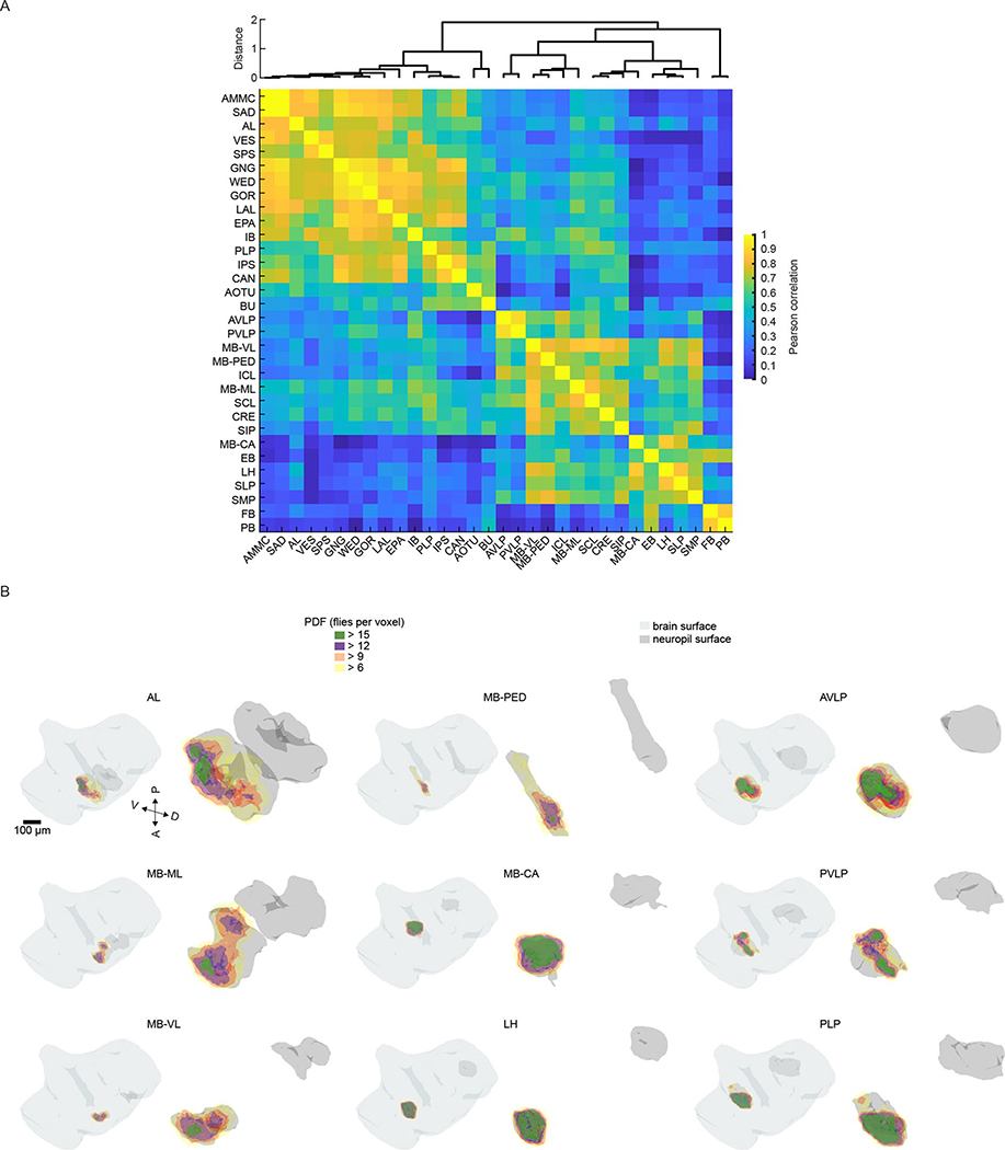
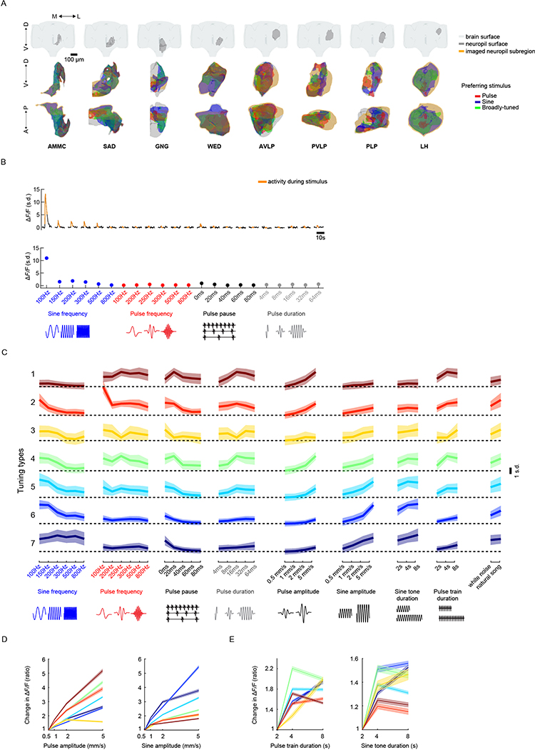
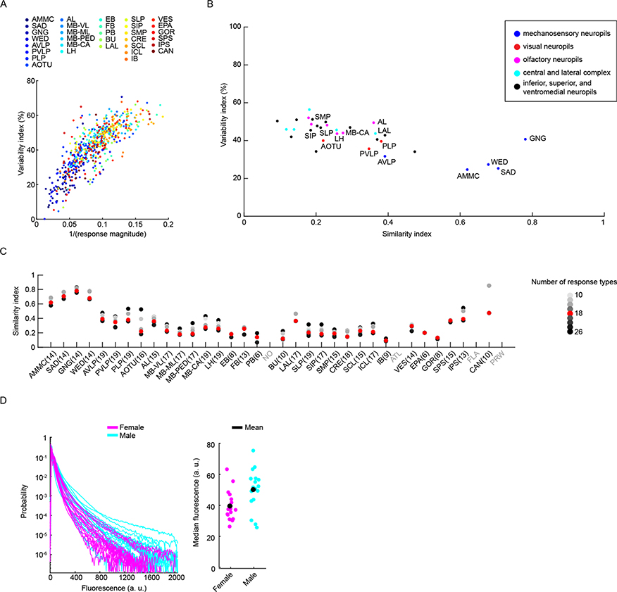
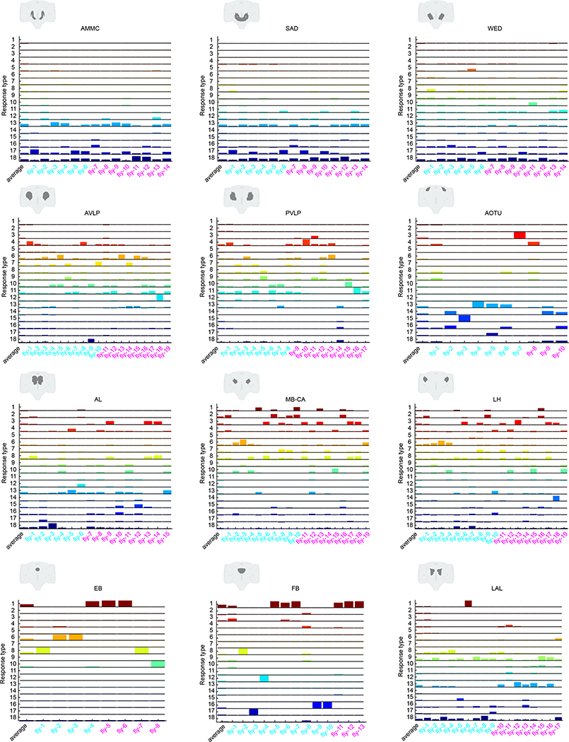
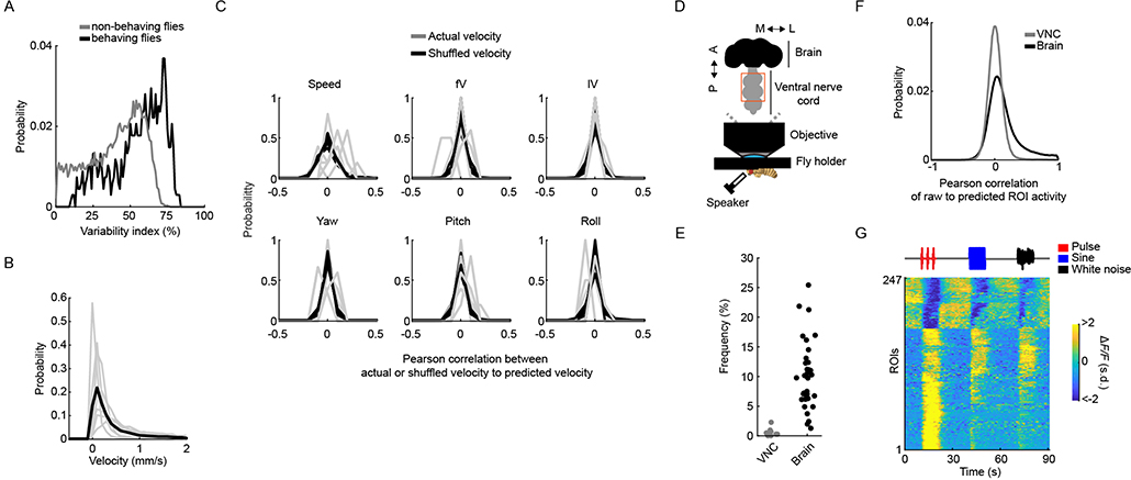
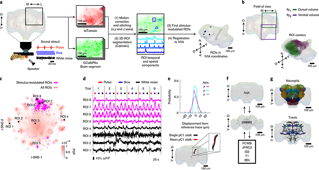
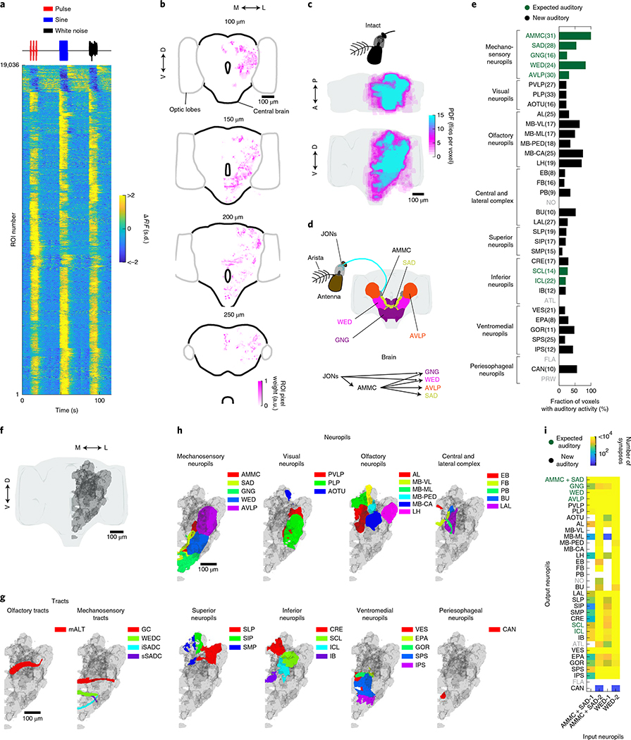
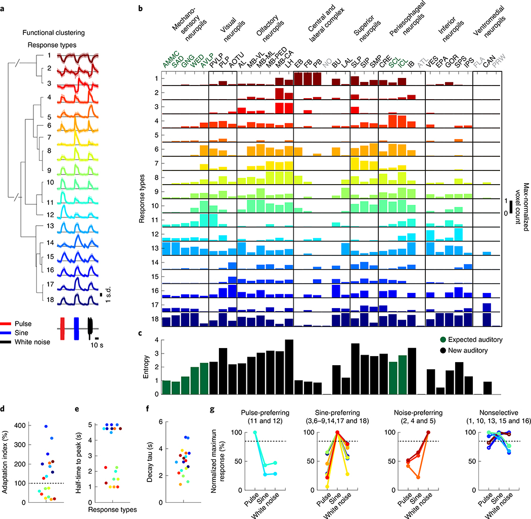
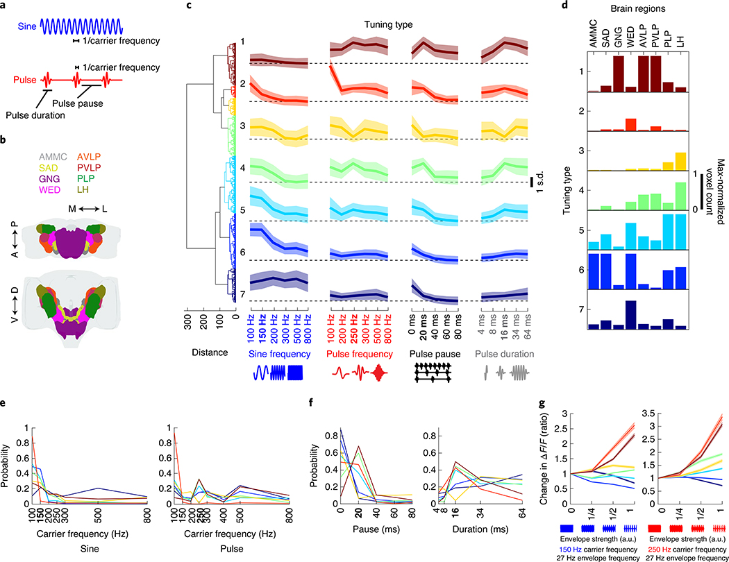
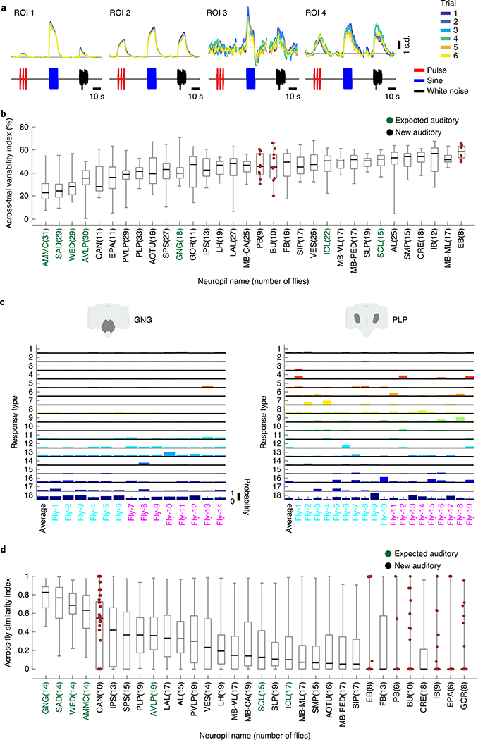
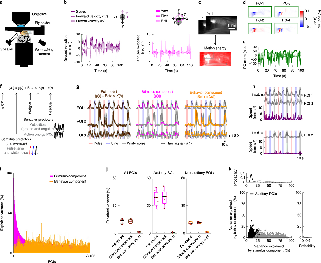
Sensory pathways are typically studied by starting at receptor neurons and following postsynaptic neurons into the brain. However, this leads to a bias in analyses of activity toward the earliest layers of processing. Here, we present new methods for volumetric neural imaging with precise across-brain registration to characterize auditory activity throughout the entire central brain of Drosophila and make comparisons across trials, individuals and sexes. We discover that auditory activity is present in most central brain regions and in neurons responsive to other modalities. Auditory responses are temporally diverse, but the majority of activity is tuned to courtship song features. Auditory responses are stereotyped across trials and animals in early mechanosensory regions, becoming more variable at higher layers of the putative pathway, and this variability is largely independent of ongoing movements. This study highlights the power of using an unbiased, brain-wide approach for mapping the functional organization of sensory activity.

Extended Data Fig. 1 |. Spatial coverage of imaged activity and measurement of auditory-evoked activity.

a, Data collection and processing. We collected data using the following protocols: a) short volumetric recordings (~10 min) of consecutive segments (from anterior to posterior axis), b) long volumetric recordings (~30 min) of selected brain areas (non-consecutive), and c) short and coarse volumetric recording (~15 min) of a single segment per fly that spans a large volume. For all these datasets we record a private whole brain structural volume (used later for registration). For all the data sets we recorded both tdTomato and GCaMP signal, and performed motion correction (using NoRMCorre) on each imaged segment using the tdTomato signal. These segments were then spatially resampled to have isotropic XY pixel size. This was followed by re-slicing of each Z-stack per segment (align time of all planes per Z-stack to the first plane imaged), and temporal resampling (aling Z-stack time relative to the start of the 1st stimulus and double the sampling rate). For protocol a), we stitched segments imaged consecutively (using NoRMCorre) obtaining a ‘volume’; for b) and c) each segment was treated as an independent volume. Volumes were mirrored to the right hemisphere, and the tdtomato signal was used for registration to the in vivo intersex atlas (IVIA). This is a two-step process, i) volumes per fly were registered to their own private whole brain volume (one per fly), and ii) whole brain volume was registered to the IVIA; registration i) and ii) were concatenated to map volumes to IVIA space. The GCaMP signal was used for ROI segmentation (via CaImAn), followed by identification of stimulus-modulated ROIs (see Extended Data Fig. 1d). b, Maximum projection (in each dimension) of segmented ROIs from all imaged volumes (n = 33 flies, 185,395 ROIs) - ROIs from the left hemisphere are mirrored (see Extended Data Fig. 1a) such that all ROIs are projected onto right hemisphere. ROIs cover the entirety of the D-V and A-P axes. Color scale indicates the number of flies with an ROI in each voxel. c, Number of ROIs across neuropils (see Fig. 1f,g and Supplementary Movies 1–4) sampled by ventral volumes or dorsal volumes (n = 33 flies, 185,395 ROIs). d, Method for identifying stimulus-modulated ROIs. Raw Ca⁺⁺ signal (F(t)) is convolved with the stimulus history (f(t)) and a set of filters per stimulus type (q(τ)) to generate the predicted Ca+ + signal. Auditory modulation is measured by the cross-validated correlation scores (⍴_F,g) between raw and predicted Ca⁺⁺ signals. Correlation of shuffled Ca⁺⁺ signal (sF(t)) to predicted signal (g(t)) is used to generate the null-distribution of correlation scores (⍴_sF,g), which is used to determine significance. e, Distribution of Pearson correlation coefficients of shuffled-vs-predicted signals (⍴_sF,g) and raw-vs-predicted signal (⍴_F,g) across all flies imaged (n = 33 flies). Unlike the distribution of ⍴_sF,g, ⍴_F,g has a distribution with a long tail of positive correlation scores. ROIs within the positive tail and outside the null distribution are considered to have significant stimuli modulation and selected as auditory ROIs. f, Frequency of auditory ROIs separated by whether the ROI was segmented from a dorsal or ventral volume (n = 33 flies).

Extended Data Fig. 2 |. Building the in vivo intersex atlas (iViA) and registering it to fixed-brain atlas (iBNWB).

a, Generation of in vivo intersex atlas (IVIA): images of male (n = 5) and female (n = 8) brains expressing membranal tdTomato pan-neuronally are registered to a seed brain (reference image). Images are then transformed to generate an average model image, which, after five iterations, produces the in vivo intersex atlas (IVIA). b, IVIA registration accuracy. Left: 3D-rendering of traced tracts of Dsx+ neurons (pC2m, pC2l), and Fru+ neuron pMP7. Right: Per-axis jitter (X, Y, and Z) between matched traced tracts of pC2m, pC2l, and pMP7 across flies (n = 10, 12, and 7 brains, respectively). c, Example imaged tdTomato volumes (red scale) from different flies registered to the IVIA (right-most column, gray scale). Middle column is the intermediate registration of volumes to their own private whole brain atlas (as in Extended Data Fig. 1a). 45 out of 48 flies were successfully registered to the IVIA. d, Central brain neuropils and tracts used for point set registration to morph the in vivo intersex atlas (IVIA) to IBNWB fixed brain atlas. Points from meshes of segmented antennal lobe (AL), mushroom body (MB) (includes mushroom body lobes, peduncle and calyx), protocerebral bridge (PB), antennal mechanosensory and motor center commissure (AMMCC), anterior optic tract (AOT), great commissure (GC), wedge commissure (WEDC), posterior optic commissure (POC), lateral antennal lobe tract (lALT), posterior cerebro-cervical fascicle (pCCF), superior saddle commissure (sSADC), and whole central brain were used to generate IVIA-to-IBNWB and IBNWB-to-IVIA transformations. e, Overlay of IVIA (red) and registered IBNWB (in IVIA space, green) at different depths (90, 130, 180, 220, 260, and 280 μm). 0 μm is the most anterior section of the brain and 300 um the most posterior. f,g, Atlas-to-atlas registration accuracy measured using pC1 stalks from IBNWB and IVIA. (f) pC1 traces from IBNWB and IVIA atlases; black traces are single pC1 neurons (from IBNWB or IVIA, n = 70 and 20 pC1 traces respectively) and red trace is the mean reference pC1 stalk. (g) Between-atlas registration accuracy; IVIA-to-IBNWB transformation increases the jitter across all axes from the reference mean pC1 trace by ~2.24 μm, while IBNWB-to-IVIA transformation increases the jitter by ~2.8 μm.

Extended Data Fig. 3 |. Auditory responses in neuropils and neurite tracts, and to additional song stimuli: natural song and fast pulses.

a, Median ROI responses (across 6 trials) to pulse, sine, and white noise stimuli (n = 33 flies, 19,036 ROIs) as in Fig. 2a, but without z-scoring ΔF/F signal. b, Spatial distribution of auditory activity across sexes. Maximum projections (from two orthogonal views) of the density of auditory ROIs in female (n = 17) or male flies (n = 16). c, Maximum projection (from two orthogonal views) of the density of i) auditory ROIs outside neuropils or neurite tracts (n = 33 flies, 4,346 ROIs), and ii) auditory ROIs within neuropils or neurite tracts (n = 33 flies, 14,658 ROIs). Color scale for (B) and (C) is the number of flies with an auditory ROI per voxel. d, Percentage of auditory ROIs within and outside neuropils and tracts, and beyond the midline. e, Spectral profile of auditory stimuli - pulse (Pslow), sine, and white noise - used to classify response types in Fig. 3a, and their spectral features. f, Spectral profile of natural song stimulus used. g, Distribution of stimuli preference (to pulse, sine, white noise, and natural song) across auditory ROIs (n = 5 flies, 2,258 ROIs). Only ~20% of auditory ROIs prefer natural song. Preference is defined by the stimulus that drives the maximum absolute response (at least 15% greater than the second highest response), as in Fig. 3f. h, Responses from auditory ROIs that prefer natural song (n = 451 ROIs). Each row is the median z-scored ΔF/F response across 6 across trials. Activity is plotted as the change in the s.d. of the ΔF/F signal. i, Spatial distribution of natural song preferring ROIs. Images are the maximum projection (from two orthogonal views) of the density of auditory ROIs with preference for natural song throughout the central brain (n = 5, 451 ROIs). j, Spectral profile of Pfast and Pslow stimuli. k, Distribution of stimuli preference to Pslow, Pfast, or broad preference for both pulse types across auditory ROIs (n = 2 flies, 2,193 ROIs). Only ~4% of auditory ROIs prefer Pfast. Preference is defined as in (G). l, Responses from auditory ROIs that prefer Pfast (n = 106 ROIs). Pfast preferring ROIs also show strong responses to Pslow. Conventions same as in (H). m, Fraction of voxels with auditory activity by central brain neurite tracts; percentages averaged across 33 flies (a minimum of 4 flies with auditory activity in a given tract was required for inclusion). Red represents tracts that were clearly distinguishable from neuropil by visual inspection (see (N)). n, For three flies, pixels with auditory activity (red) overlaid on time-averaged GCaMP6 fluorescence (grayscale). Several neurite tracts are indicated (planes from different depths are arbitrarily selected for each fly to highlight ROIs contained within neurite tracts).

Extended Data Fig. 4 |. Auditory activity is present in olfactory pathway neurons and absent in deaf flies.

a,b, Auditory responses from (A) putative individual antennal lobe projection neurons (PNs), and (B) putative individual mushroom body Kenyon cells (KCs) from pan-neuronal recordings. Time-averaged GCaMP6s signal is shown in grayscale (over the entire experiment). Pixels belonging to individual ROIs and their corresponding time traces (median z-scored ΔF/F responses across 6 trials to pulse, sine, and white noise stimuli) are indicated in different colors. ROIs were drawn manually over the location of PN or KC somas from two independently imaged flies. Activity scale bar unit is s.d. c,d, Auditory responses from (C) antennal lobe projection neurons, and (D) mushroom body Kenyon cells using cell type specific genetic lines (GH146-Gal4 and OK107-Gal4, respectively). Time-averaged GCaMP6s signal is shown in grayscale (over the entire experiment) - the compartments where activity was recorded from are indicated (data was collected and processed as we did for pan-neuronal data (protocol a) in Extended Data Fig. 1a) but the field of view was restricted to the region defined by the orange and purple boxes). Auditory ROIs are detected in all imaged compartments of antennal lobe projection neurons (n = 8 flies, 1,133 ROIs) and Kenyon cells (n = 4 flies, 154 ROIs). Each row is the median across 6 trials - all responses are z-scored and therefore plotted as the change in the s.d. of the ΔF/F signal. e, Number of detected auditory ROIs per fly in wild type (n = 33 flies) and iav¹ flies (n = 4 flies). f, Maximum projection (from two orthogonal views) of the density of auditory ROIs in iav¹ flies (all 21 ROIs come from 1 out of 4 flies imaged). These few ROIs were located in the mushroom body calyx (MB-CA), posterior VLP (PVLP), and the posterior lateral protocerebrum (PLP). Color scale is the number of flies with an auditory ROI per voxel. g, Distribution of mean ΔF/F values (during stimuli) for auditory ROIs in wild type (n = 33 flies) and iav¹ flies (n = 4 flies).

Extended Data Fig. 5 |. Auditory responses are not sexually dimorphic and Auditory response types have distinct spatial distributions throughout the central brain.

a, Hierarchical clustering of auditory responses into 18 distinct response types, and divided by sex. The mean response across ROIs belonging to each response type is shown. All responses are z-scored (as in Fig. 3a), and therefore plotted as the s.d. of the responses over time. Color code is the same as in Fig. 3a. b, Probabilities of neuropil voxels with a given response type (separated by sex) in two neuropils, the gnathal ganglion (GNG) and the lateral accessory lobe (LAL). These are the only two neuropils with sex differences - males have a slightly higher probability of response type 18 activity in the GNG, while females have a slightly higher probability of response type 13 activity in the LAL. Each dot is the probability for one fly. c, Sex-related differences in all response types across all neuropils. Each dot is the effect size (see Methods) of the difference in probability for each response type across sexes, color code is the same as (A). Neuropils with the greatest effect size are the GNG (response type 18) and LAL (response type 13). However all differences are not significant (p > 0.05). Statistical significance was determined using two-tailed two-sample t-test with Benjamini-Hochberg FDR correction. Neuropils with no auditory activity are indicated in gray font. d, Spatial distribution of excitatory vs inhibitory auditory ROI responses across the central brain. Images are the maximum projection (from two orthogonal views) of the density of excitatory and inhibitory responses across flies (n = 33 flies). e, Spatial distribution of auditory activity belonging to each response type (see Fig. 3a) across the central brain. Images are the maximum projection (from two orthogonal views) of the density of responses across flies for each response type (n = 33 flies). Color scale for (D) and (E) is the number of flies with an auditory ROI belonging to each category (excitatory, inhibitory, or response type) per voxel.

Extended Data Fig. 6 |. Similarity of auditory activity between neuropils, and compartmentalization within neuropils.

a, Pairwise Pearson’s correlation coefficients of response type distributions (as in Fig. 3b) between neuropils. Neuropils are ordered based on the hierarchical clustering of the correlation matrix. Only positive correlation values are plotted for clarity. b, Spatial distribution of auditory responses within selected olfactory (AL, MB-ML, MB-VL, MB-PED, MB-CA, and LH), visual (PVLP, and PLP) and mechanosensory neuropils (AVLP). Auditory activity is spatially restricted within each neuropil. Voxel density was calculated from 19, 15, 17, 17, 22, 19, 18, 30, and 25 flies for the AL, MB-ML, MB-VL, MB-PED, MB-CA, LH, PVLP, PLP, and AVLP respectively.

Extended Data Fig. 7 |. Neuropil subregions imaged, definition of stimulus tuning, and tuning for additional song features.

a, Neuropil volume and subregion of neuropil imaged in Fig. 4. Top row, location of the neuropil imaged (dark grey surface) relative to the central brain (light grey surface). Middle and bottom rows show maximum projections (from two orthogonal views) of imaged neuropil subvolume (orange surface) and the distribution of ROI stimulus selectivity (based on data in Fig. 3b). The neuropil subvolume (orange) is the volume imaged in at least 2 flies. This volume represents 24.4, 46.2, 10.5, 83, 39.8, 99.3, 63.6, and 91.8 % of the AMMC, SAD, GNG, WED, AVLP, PVLP, PLP and LH, respectively. b, Example responses from one ROI to song feature stimuli (see Fig. 6a). Top panel, Median (across trials) and z-scored responses to each song feature (responses are baseline subtracted, and baseline is defined as activity −4 to −0.25 seconds before stimulus onset). Orange timepoints correspond to activity during the stimulus. Bottom panel, response magnitudes (80th or 20th percentile of activity - for excitatory or inhibitory responses - during stimulus plus 2 seconds after) to each song feature calculated from the top trace (that is the tuning curve for this ROI). All responses are z-scored, so responses are plotted as the s.d. of ΔF/F value. c, Tuning types as in Fig. 6c, but plotting additional responses to pulses and sines of different amplitudes, varying pulse and sine train durations, and also to white noise and natural song (these additional responses were not used to cluster responses). Thick traces are the mean response magnitudes (calculated as in (B)) across all ROIs within each tuning type and shading is the standard deviation (1,783, 513, 739, 1,682, 2,410, 2,321 and 1424 ROIs for each tuning type 1–7 respectively, n = 21 flies). Responses are plotted as the s.d. of ΔF/F value. d, Auditory responses to different sine and pulse intensities, sorted by tuning type. Response magnitudes (calculated as in (B), but 80th or 20th percentile of the activity is measured during stimuli only) per ROI are normalized to the response to 0.5 mm/s stimuli. Thick traces are the mean normalized response magnitude, and shading is the s.e.m (ROI number per tuning type is the same as in (C)). e, Auditory responses to different sine and pulse train durations. Response magnitudes (calculated as in (D)) per ROI are normalized to the response to 2 seconds stimuli. Conventions same as in (D).

Extended Data Fig. 8 |. Across-trial and across-individual comparisons of auditory activity by neuropil.

a, Comparison of across-trial variability index (see Fig. 5b) and response magnitude. Each dot is the mean variability index and response magnitude (80^th or 20^th percentile - for excitatory or inhibitory responses - of z-scored ΔF/F from stimuli onset until 5 seconds after stimulus offset) per neuropil for each fly (across all ROIs). Neuropils are color coded according to the legend. Variability index is inversely correlated with response magnitude. b, Comparison of across-trial variability (see Fig. 5b) and across-individual similarity (see Fig. 5d). Each dot is the mean across-trial variability index and mean across-individual similarity index per neuropil. Groups of neuropils are color coded according to the legend. Early mechanosensory neuropils have low across-trial variability and high across-individual similarity. c, Robustness of differences in similarity index across neuropils to the number clusters selected for hierarchical clustering of response types (see Fig. 3a). Similarity index per neuropil (as in Fig. 5d) is calculated for different numbers of clusters (from 10 to 26 - in Fig. 3 we used 18 types (red)). d, No systematic difference in distribution of time-average fluorescence (over the entire experiment) across individuals. Left: Histograms of time-averaged fluorescence per individual, cyan and magenta correspond to male (n = 16) and female (n = 17) flies. Right: Median fluorescence per individual. Black dot corresponds to the mean (of median fluorescence) across flies.

Extended Data Fig. 9 |. Distribution of 18 auditory response types per neuropil, separated by flies.

Response type distributions, similar to Fig. 5c, for mechanosensory, visual, olfactory, central and lateral complex neuropils. For each neuropil, male and female flies are indicated in cyan or magenta, respectively.

Extended Data Fig. 10 |. Behavior of head-fixed flies and minimal auditory responses in the Drosophila ventral nerve cord.

a, Distribution of across-trial variability of auditory ROIs in behaving (data used in Fig. 6, n = 7 flies, 4,560 ROIs) and non-behaving flies (data used in Fig. 5b, n = 33 flies, 19,036 ROIs). b, Distribution of speed across flies. Each gray line is the speed distribution per fly (n = 7 flies), and black line is the mean across animals. c, Correlation between linearly predicted velocities (based on stimuli history) and actual or shuffled (see Methods) velocities. Each black or gray line is the probability per fly (n = 7 flies). d, Schematic of VNC functional imaging during auditory stimulation. Similar to Fig. 1a, but the dorsal side of the thorax is dissected to expose the dorsal side of the first and second segment of the VNC depicted inside the orange rectangle. e, Frequency of auditory ROIs detected in the brain (n = 33 flies, 185,395 ROIs) and the VNC (n = 8 flies, 39,580 ROIs) using the same criteria as in Extended Data Fig. 1d. f, Distribution of Pearson correlation coefficients of raw ROI activity to predicted ROI activity (based on stimuli history, as in Extended Data Fig. 1e) for ROIs recorded from the brain (n = 33 flies, 185,395 ROIs) and the VNC (n = 8 flies, 39,580 ROIs). g, Responses of VNC auditory ROIs to pulse, sine, and white noise stimuli (n = 8 flies, 39,580 ROIs). Each row is the across-trial median and z-scored ΔF/F response to each stimulus (6 trials per stimulus). ΔF/F units are in s.d.

Fig. 1 |. A new pipeline for mapping sensory activity throughout the central brain.

a, Overview of data collection and processing pipeline (for more details see Extended Data Fig. 1a). Step (1): the tdTomato signal is used for motion correction of a volumetric time-series and to stitch serially imaged overlapping brain segments in the x, y and z axes. Step (2): 3D ROI segmentation (via CaImAn) is performed on GCaMP6s signals. Step (3): auditory ROIs are selected. Step (4): ROIs are mapped to the in vivo intersex atlas (IVIA) space. D, dorsal; L, lateral; M, medial; V, ventral. b, Top: an example of 11,225 segmented ROIs combined from two flies (dorsal (green) and ventral (purple) volumes from each fly). Bottom: ROI centers (dots) span the entire anterior–posterior (A–P) and D–V axes. These ROIs have not yet been sorted for those that are auditory (Extended Data Fig. 1d,e). c, 2D t-SNE embedding of activity from all ROIs in b. PDF, probability density function. ROIs modulated by auditory stimuli (1,118 out of 11,225 ROIs) are shown in magenta. d, ΔF/F from ROIs indicated in c. Magenta traces correspond to stimulus-modulated ROIs, while black traces are non-modulated ROIs. Time of individual auditory stimulus delivery is indicated (pulse, sine or band-limited white noise). e, Top: IVIA registration accuracy showing the per-axis jitter (x, y and z) between traced pC1 stalk values across flies relative to mean pC1 stalk values (see Extended Data Fig. 2a–c for more details). Bottom: 3D rendering of traced stalks of Dsx⁺ pC1 neurons (black traces, n = 20 brains from Dsx–GAL4/UAS–GCaMP6s flies) and mean pC1 stalk (red trace). f, Schematic of the bridging registration between the IVIA and the Insect Brain Nomenclature Whole Brain (IBNWB) atlas. This bidirectional interface provides access to a network of brain atlases (FCWB, JFRC2, IS2, T1 and IBN) associated with different Drosophila neuroanatomy resources. See Extended Data Fig. 2d–g for more details. g, Anatomical annotation of the IVIA. Neuropil and neurite tract segmentations from the IBN atlas were mapped to the IVIA (for a full list of neuropil and neurite tract names, see Supplementary Table 1). See also Supplementary Videos 1–4.

Fig. 2 |. Auditory activity is widespread throughout the central brain of Drosophila.

a, Auditory ROI responses to pulse, sine and white noise stimuli (n = 33 flies, 19,036 ROIs). Each row is the median across six trials, with all responses z-scored and therefore plotted as the change in the s.d. of the ΔF/F signal. ROIs are sorted on the basis of clustering of temporal profiles (Fig. 3a). b, The spatial distribution of auditory ROIs (ROI pixel weights (arbitrary units (a.u.) in magenta) combined from two flies (one ventral and one dorsal volume) (ROIs are in IVIA coordinates). Four different depths are shown (0 μm is the most anterior section of the brain and 300 μm the most posterior). The gray contour depicts the optic lobes, while the black contour depicts the central brain. c, Maximum projection (from two orthogonal views) of the density of auditory ROIs (n = 33 flies, 19,036 ROIs). The color scale represents the number of flies with an auditory ROI per voxel. d, Schematic of the canonical mechanosensory pathway in D. melanogaster. JONs in the antenna project to the AMMC, the GNG and the WED. AMMC neurons connect with the GNG, the WED, the SAD and the AVLP. e, The fraction of voxels with auditory activity by central brain neuropil. Percentages are averaged across 33 flies (a minimum of 4 flies with auditory activity in a given neuropil was required for inclusion). The number of flies with auditory responses in each neuropil are indicated in parentheses. Neuropils with no auditory activity are indicated in gray font (also for i). f–h, 3D rendering of the volume that contains all auditory voxels across all flies (gray) (f) and the overlap of this volume with tracts (g) and brain neuropils (h). i, Using the hemibrain connectomic dataset, a heatmap was generated of neuropils in which all identified AMMC/SAD or WED neurons (1,079 and 3,556, respectively) have direct synaptic connections (AMMC+SAD-1 or WED-1) and neuropils with connections to AMMC/SAD or WED neurons via one intermediate synaptic connection (AMMC+SAD-2 or WED-2). Neuropils with fewer than five synapses are shaded white. See also Extended Data Figs. 3 and 4 and Supplementary Video 5. For a full list of neuropil and neurite tract names, see Supplementary Table 1.

Fig. 3 |. Brain-wide auditory activity is characterized by a diversity of temporal response profiles across neuropils.

a, Hierarchical clustering of auditory responses into 18 distinct response types (Methods). Thick traces are the mean response (across ROIs) to pulse, sine and white noise, and shading is the s.d. (n = 33 flies, 19,036 ROIs). All responses are z-scored, and therefore plotted as the s.d. of the responses over time, with the black dash line corresponding to the mean baseline across stimuli for each response type. b, Distribution of 18 response types across 36 central brain neuropils. The histogram of voxel count (how many voxels per neuropil with auditory activity of a particular response type) was max-normalized for each neuropil (normalized per column). The color code is the same as in a (n = 33 flies). Neuropils with no auditory activity are indicated in gray font. c, The diversity (measured as the entropy across response-type distributions shown in b) of auditory responses across central brain neuropils (Methods). d–f, Kinetics of all auditory responses by response type. Adaptation (d), half-time to peak (e) and decay time tau (f). g, Diversity in tuning for response types showing pulse-preferring, sine-preferring, noise-preferring and nonselective response types (preference is defined by the stimulus that drives the maximum absolute response (at least 15% greater than the second highest response). Nonselective responses are divided into sine-and-pulse-preferring (filled circles) and sine-and-noise-preferring (open circles). See also Extended Data Figs. 5 and 6.

Fig. 4 |. Widespread auditory activity is tuned to features of conspecific courtship songs.

a, Spectral and temporal features of the two main modes of Drosophila courtship song. b, Neuropils imaged. c, Hierarchical clustering of auditory tuning curves (see Extended Data Fig. 7a for how tuning curves were generated) into seven distinct tuning types. Tuning types 1–7 comprise 1,783; 513; 739; 1,682; 2,410; 2,321 and 1,424 ROIs, respectively (n = 21 flies). Thick traces are the mean z-scored response magnitudes (80th or 20th percentile of activity—for excitatory or inhibitory responses—during stimuli plus 2 s after. Activity is plotted as the s.d. of ΔF/F values to the stimuli indicated on the x axis (across ROIs and within each tuning type) and shading is the s.d. (across ROIs within tuning type). D. melanogaster conspecific values of each courtship song feature are indicated in bold on the x axis (same for e and f). d, Distribution of tuning types across regions of selected brain neuropils imaged. The histogram of voxel count per type (number of voxels with activity that falls into each tuning type) was max-normalized for each neuropil (normalized per column). e, Probability distributions of best frequency for sine and pulse, separated by tuning type. The color code is the same as in c. f, Probability distributions of best pulse duration and pulse pause. Conventions are the same as in e. g, Effects of the amplitude envelope on responses to sine tones. Envelopes (~27-Hz envelope) of different amplitudes were added to sine tones (as depicted on the x axis; see Methods for more details) of 150 or 250 Hz. ROI response magnitudes to different envelope strengths were normalized to responses to envelope strength 0 (that is, a sine tone of 150 or 250 Hz, with no envelope modulation) and sorted by tuning type from c. Thick traces are the mean-normalized response magnitudes per tuning type, and shading is the s.e.m. (ROI number per tuning type is the same as in c). See also Extended Data Fig. 7.

Fig. 5 |. Auditory activity is more similar across trials and individuals in early mechanosensory areas.

a, Example auditory responses from five different ROIs to pulse, sine and white noise stimuli. Individual trials are plotted in different colors. All responses are z-scored, and therefore plotted as the s.d. of the responses over time, with the black dashed line corresponding to the mean baseline across stimuli for each ROI. b, The across-trial variability index of individual ROIs was computed as the residual of the variance explained by the mean across trials (Methods). The gray box shows the 25th and 75th percentile, the inner black line is the median variability across flies (number of flies per neuropil are shown in parentheses), and the whiskers correspond to minimum and maximum values. If n < 11, we plot means per fly with brown dots. c, Stereotypy of auditory response types (Fig. 3a,b) across individuals for the GNG and the PLP. Male flies are indicated in cyan and female flies in magenta on the x axis. Auditory activity in the GNG is similar across flies, while auditory activity in the PLP is more variable, in terms of response type diversity. Average response across all flies is shown in the left-most column. d, The across-individual similarity index was computed by measuring the cosine between response type distributions (Fig. 3b) per neuropil across individuals (Methods). Conventions are the same as in b. For each neuropil, we computed the similarity index for all possible pairs of flies. Responses in the GNG, SAD, WED and AMMC are the most stereotyped across individuals. See also Extended Data Figs. 8 and 9.

Fig. 6 |. Spontaneous movements do not account for trial-to-trial variability in auditory responses.

a, Schematic of the functional-imaging protocol of a head-fixed fly walking on a ball. b, Instantaneous ground and angular velocities measured from ball tracking of a representative tethered fly walking. c, Motion energy (absolute value of the difference of consecutive frames) from a video recording of tethered fly. Gray contours correspond to pixels excluded from analysis (Methods). d, Coefficients of the top four principal components (PCs) of the motion energy movie (image scale represents low-motion (blue) to high-motion energy (red)) of a representative tethered fly (same as b). e, Scores of the top four PCs of the motion energy movie (the color of each PC is the same as in box color in d) of a representative tethered fly (same as b). f, Schematic of the linear model used to predict neural activity related to either stimuli or behavior. ROI activity (y(t)) is modeled as the sum of the stimulus component (trial average, μ(t)), behavior component (Beta × X(t)), plus noise (ε(t)). g, ROI activity along with predictions by stimulus component (μ(t)), behavior component (Beta × X(t)) or the full model for three example ROIs most strongly modulated by auditory stimuli (ROI 1), by behavior (ROI 2) or by the combination of both (ROI 3). The ROI activity values were z-scored, and ΔF/F units are in s.d. (also for h). h, Activity of ROIs from g along with speed. ROIs from the same fly are plotted together. i, Explained variance by stimulus component or behavior component for individual ROIs, sorted by stimuli-only model performance (n = 7 flies, 63,106 ROIs). j, Mean explained variance by stimulus component (μ(t)), behavior component (Beta × X(t)) or both (μ(t) + Beta × X(t)) across flies, for all ROIs (left), auditory ROIs only (middle) and non-auditory ROIs (right). The box shows the 25th and 75th percentile, the inner black line is the median explained variance across flies, and whiskers correspond to minimum and maximum values. Means per fly are plotted with brown dots (n = 7 flies). k, Explained variance by stimulus component versus behavior component for individual ROIs. Gray dots correspond to auditory ROIs (using the same criteria as in Extended Data Fig. 1d). See also Extended Data Fig. 10.

References

1. Mann K, Gallen CL & Clandinin TR Whole-brain calcium imaging reveals an intrinsic functional network in Drosophila. Curr. Biol 27, 2389–2396.e4 (2017). - PMC - PubMed
1. Chen X et al. Brain-wide organization of neuronal activity and convergent sensorimotor transformations in larval zebrafish. Neuron 100, 876–890.e5 (2018). - PMC - PubMed
1. Bates AS et al. The natverse, a versatile toolbox for combining and analysing neuroanatomical data. eLife 9, e53350 (2020). - PMC - PubMed
1. Deutsch D, Clemens J, Thiberge SY, Guan G & Murthy M Shared song detector neurons in Drosophila male and female brains drive sex-specific behaviors. Curr. Biol 29, 3200–3215.e5 (2019). - PMC - PubMed
1. von Schilcher F The role of auditory stimuli in the courtship of Drosophila melanogaster. Anim. Behav 24, 18–26 (1976).
Publication types
LinkOut - more resources