Review
. 2021 Jan 15:348:109007.
doi: 10.1016/j.jneumeth.2020.109007. Epub 2020 Nov 23.

Gradient waveform design for tensor-valued encoding in diffusion MRI

Affiliations
Review

Gradient waveform design for tensor-valued encoding in diffusion MRI

Filip Szczepankiewicz et al. J Neurosci Methods. .

Abstract

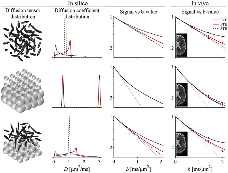
Diffusion encoding along multiple spatial directions per signal acquisition can be described in terms of a b-tensor. The benefit of tensor-valued diffusion encoding is that it unlocks the 'shape of the b-tensor' as a new encoding dimension. By modulating the b-tensor shape, we can control the sensitivity to microscopic diffusion anisotropy which can be used as a contrast mechanism; a feature that is inaccessible by conventional diffusion encoding. Since imaging methods based on tensor-valued diffusion encoding are finding an increasing number of applications we are prompted to highlight the challenge of designing the optimal gradient waveforms for any given application. In this review, we first establish the basic design objectives in creating field gradient waveforms for tensor-valued diffusion MRI. We also survey additional design considerations related to limitations imposed by hardware and physiology, potential confounding effects that cannot be captured by the b-tensor, and artifacts related to the diffusion encoding waveform. Throughout, we discuss the expected compromises and tradeoffs with an aim to establish a more complete understanding of gradient waveform design and its impact on accurate measurements and interpretations of data.

Keywords: Diffusion magnetic resonance imaging; Gradient waveform design; Tensor-valued diffusion encoding.


Figures

Fig. 1.
Fig. 1.
A variety of gradient waveform designs and their dephasing vector trajectory in a spin-echo sequence. For comparability, all waveforms are adapted to yield b = 2 ms/μm2 at a minimal encoding time limiting the maximal gradient amplitude and slew rate to 80 m T/m and 100 T/m/s. We assume that the refocusing pulse lasts 8 ms and the encoding duration after the refocusing is 6 ms shorter than the duration before (δ1 = δ2 + 6 ms). Columns, from left to right, show the effective gradient waveform, the physical gradient trajectory, the dephasing q-vector trajectory, and a table of characteristics related to the b-tensor shape (Section 2.1), optimization norm (Section 3.1), concomitant gradient compensation (Section 5.2), encoding efficiency (κ, Section 2.3) and relative energy consumption (Erel, Section 3.2), as described throughout the paper. The monopolar pulsed field gradient by Stejskal and Tanner (1965) yields diffusion encoding along a single direction, also called linear b-tensor encoding (LTE). The waveform used by Cory et al. (1990) combines two orthogonal pairs of bipolar pulses to yield planar b-tensor encoding (PTE). This design allows arbitrarily directions for the two pairs and can therefore yield b-tensor shapes between LTE and PTE. Waveforms by Mori and van Zijl (1995); Wong et al. (1995); Heid and Weber (1997); Chun et al. (1998) and Topgaard (2013) were all designed to yield spherical b-tensor encoding (STE). The design by Lasic et al. (2020) can produce motion compensation of arbitrary order, and remaining designs by Sjölund et al. (2015); Szczepankiewicz et al., 2019 generate optimal waveforms tailored to a given MRI system and sequence setup (only STE is shown). As indicated by the total duration next to the waveforms, the encoding efficiency varies widely (shorter times are more efficient). Note that we modified ‘pattern I’ in Mori and van Zijl (1995), denoted PI*, to improve its efficiency and yield compensation for concomitant gradient effects (K-nulling, Section 5.2). The waveform by Wong et al. (1995) was split in two parts and placed around the refocusing pulse, according to the implementation in Butts et al. (1997). Finally, we note that the waveform by Heid and Weber (1997) is the basis for the ‘one-scan-trace’ design found at Siemens MRI systems (Dhital et al., 2018).
Fig. 2.
Fig. 2.
The shape of the b-tensor influences the effect of diffusion anisotropy on the signal. The in silico examples show three diffusion tensor distributions, P(D), with corresponding distributions of apparent diffusion coefficients, P(D) = P((B/b) : D). From top to bottom they are randomly oriented anisotropic tensors; mixture of isotropic tensors with fast and slow diffusion; and mixture of anisotropic and isotropic diffusion tensors. The second column shows the effective distribution of apparent diffusion coefficients observed when using linear (LTE, solid black lines), planar (PTE, red lines) and spherical b-tensors (STE, broken black lines). The different distributions of diffusion coefficients manifest as different signal vs b-value curves (Eq. (9)). For sufficiently large b-values, the signal is non-monoexponential in the presence of multiple diffusivities. Although this condition can be caused by markedly different diffusion tensor distributions, the three examples are indistinguishable if we can only make use of conventional diffusion encoding (Mitra, 1995; Szczepankiewicz et al., 2016). However, we may complement the measurement with b-tensors that have multiple shapes to isolate the contribution from microscopic diffusion anisotropy. This is the central motivation for using tensor-valued diffusion encoding. From a phenomenological perspective, the hallmark of ‘microscopic diffusion anisotropy’ is diverging signal between STE and all other b-tensor shapes, and the hallmark of ‘heterogeneous isotropic diffusion’ is non-monoexponential STE signal. The in vivo examples show similar signal behavior in three regions of healthy brain parenchyma, and it is the purpose of models and representations to infer the microstructure from the signal (Novikov et al., 2018a). The in vivo data used in this example is available online (Szczepankiewicz et al., 2019a).
Fig. 3.
Fig. 3.
Encoding efficiency (κ, Eq. (10)) as a function of the total encoding time. The general trend is that linear encoding is the most efficient, followed by planar and spherical variants. Waveforms that are constrained by the max-norm (broken lines) have superior efficiency than those constrained by the L2-norm (solid lines, see Section 3.1). However, we note that max-norm optimization does not allow arbitrary waveform rotation (Fig. 4). Therefore, we show the max-norm only for spherical b-tensor encoding since they may not require any rotation. Furthermore, ‘Maxwell-compensated’ waveforms (black lines) have slightly lower efficiency compared to waveforms that may suffer errors from concomitant gradients (red lines) as described in Section 5.2. For example, compare numerically optimized waveforms by Sjölund et al. (2015) and Szczepankiewicz et al., 2019. The labels m1 and m2 indicate velocity and acceleration-compensation, respectively (Section 4.3). Diagonal gray lines intersect the efficiency lines of each design at points where they yield b-values between 0.5 and 8 ms/μm2. Although the optimal gradient waveform design is largely determined by the specifics of the application, the most versatile designs use the L2-norm and compensation for concomitant gradient effects (solid black lines). Finally, the impact of finite slew-rates can be seen as the amount of efficiency that is lost as the total encoding duration is reduced; waveforms that spend longer on slewing are the most affected (Sjölund et al., 2015).
Fig. 4.
Fig. 4.
Waveforms optimized with constraints on the L2-norm (Euclidean) and max-norm allow for different rotations. The gradient waveform on the left is inscribed within a sphere and can be freely rotated without violating the maximal gradient amplitude limitations. By contrast, the waveform on the right is inscribed within a cube and will therefore protrude through its surface when rotated. Naturally, the max-norm still allows for rotations in steps of 90° around the x, y and z-axes, as well as axis permutations. In cases where the b-tensor does not have to be rotated, e.g., when we may assume that spherical b-tensor encoding is rotation invariant, the max-norm may provide a significant performance boost compared to the L2-norm. In this example, waveforms were numerically optimized (Sjölund et al., 2015; Szczepankiewicz et al., 2019) to the conditions described in Fig. 1, and yield b = 2 ms/μm2 in 73 ms and 56 ms, respectively. Naturally, any waveform that exceeds the capacity of the gradient amplitude or slew rate may be scaled down, or de-rated, to be within specifications, although this is at a cost to performance (Eq. (10)).
Fig. 5.
Fig. 5.
The order of diffusion encoding determines the peak thermal load on the system. The sorted method uses four b-values executed in order, from low to high. The interleaved sampling schemes acquire the same b-values, but each consecutive volume or slice uses a different b-value. Similarly, the random sampling acquires consecutive slices with random diffusion weighting between 0.1 and 2.0 ms/μm2. The figure shows that the peak thermal load is the largest when samples are acquired in order, i.e., executing the highest b-value many times in a row tends to heat the system in an unfavorable way compared to interleaved schemes (Hutter et al., 2018a). This example is based on Newton’s law of cooling (Newton, 1701) for a hypothetical imaging setup that uses 60 slices per volume, 4 b-values, 10 repetitions per b-value, shots separated by 125 ms, and a system with a cooling time constant ln(2)/30 s−1.
Fig. 6.
Fig. 6.
Peripheral nerve stimulation (PNS) levels vary over time and are induced by rapid and sustained switching of the gradients. The plots on the left show waveforms with the highest peak and cumulative PNS among the tested waveforms, respectively. From the slew rate diagrams (second row), it is clear that high PNS occurs when gradients transition between maximal positive to negative gradients. We emphasize that all waveforms were limited to use the same maximal slew rate, yet they cover a wide range of PNS levels, as seen in the right plot. The PNS can be reduced by limiting the maximal slew rate for the whole waveform, or by limiting the slew rate in segments where switching is sustained for longer periods of time and/or in short succession. Moreover, the PNS response may depend on subject position or waveform rotation (Budinger et al., 1991; Lee et al., 2016). For example, the waveform on the left creates a larger peak PNS on the y-axis (gray) compared to the z-axis (red), even if the bipolar pairs are otherwise identical. In this figure, PNS values were calculated to visualize representative PNS response functions, the wide range of possible values, and the rotation variance using an in-house implementation (https://github.com/filip-szczepankiewicz/safe_pns_prediction) of the SAFE model (Hebrank and Gebhardt, 2000) assuming a representative MRI system.
Fig. 7.
Fig. 7.
The b-tensor describes encoding for Gaussian diffusion but most gradient waveforms also encode for features beyond the b-tensor. The first two columns visualize the effect of diffusion time where diffusion is restricted inside a one-dimensional stick with length l. The first column shows the apparent diffusion coefficients as a function of stick length and rotation; the inset glyph shows the apparent diffusivity for sticks with length l = 20 μm directed along multiple directions. The second column shows the waveforms and encoding power spectra associated with the highest (red) and lowest (black) apparent diffusivity and encoding frequency. The trend is that faster gradient oscillations have more power at higher frequencies, equivalent to shorter diffusion times, and therefore detect a higher apparent diffusivity (Stepisnik, 1993). The third column shows a similar analysis of the exchange weighting time (Γ in Eq. (24)) (Ning et al., 2018). The glyphs show the exchange weighting along multiple directions, and the plotted waveforms are those that create the longest (red) and shortest (black) exchange times. In the final column, we show the vector-valued velocity encoding (m1 in Eq. (25)) (Nalcioglu et al., 1986). Again, the sub-selected waveforms show maximal (red) and minimal (black) velocity encoding. For the selected example waveforms, we observe that diffusivity measured by DDE is relatively isotropic, even if the encoding power spectra are markedly different (similar bVω in Eq. (23)). By contrast, the exchange weighting and velocity encoding are highly anisotropic. The waveform by Chun et al. (1998) has anisotropic diffusion time and exchange characteristics, but is velocity compensated." Also remove the reference to Section 5.4. Finally, the design by Szczepankiewicz et al., 2019 has a superior encoding efficiency and is compensated for concomitant gradients (Section 5.2), but exhibits the highest spectral anisotropy.
Fig. 8.
Fig. 8.
The desired gradient waveform is always accompanied by concomitant gradients such that the actual gradient waveform is the sum of the two. Even if the desired gradient waveform is balanced, the concomitant waveform may not be, and their residual moment (qc(τ)=k~) causes image artifacts that run the gamut between imperceptible to complete signal dropout. The columns, from left to right, show the desired gradient waveforms in different rotations (R g(t)), their concomitant gradient waveforms (gc(t)) and magnitude of the dephasing vector trajectory (∣qc(t)∣) at position r = [7 7 7] cm, glyphs of the residual dephasing vector k~ for an exhaustive set of waveform rotations, and signal maps in an oil phantom (Szczepankiewicz et al., 2019). The first row shows double diffusion encoding where the gradient pulses are both in the x-y-plane. In this special case, the concomitant gradients cancel due to a symmetry in the contribution from the x and y axes (Eq. (29)), and the dephasing vector at the end of encoding is negligible. By contrast, all other rotations result in a non-zero dephasing vector. For the worst rotation (middle row), this may result in a complete loss of signal, as seen 7 cm from the isocenter. In this oil phantom, the signal attenuation due to diffusion weighting is negligible, therefore, the severe signal attenuation in the middle row is an artifact caused by concomitant gradients. Note that this applies to the double diffusion encoding in a single spin-echo but can be avoided in double spin-echo sequences. Using an identical imaging setup, the worst rotation for a ‘Maxwell-compensated’ waveform has a negligible dephasing vector and no observable loss of signal (bottom row). Note that the glyphs show the residual dephasing for several orientations of the symmetry axis using the rotation method described in Szczepankiewicz et al. (2019a), where a final rotation around the symmetry axis is applied to find the worst case scenario. Details about the experiments and open source tools (https://github.com/markus-nilsson/md-dmri/tree/master/tools/cfa) for analysis of concomitant gradients and their effects can be found in Szczepankiewicz et al., 2019.
Fig. 9.
Fig. 9.
The effect of background gradients will depend on their interaction with the desired gradient waveforms. The plots show three variants of double diffusion encoding waveforms in a spin-echo, and we introduce an exaggerated background gradient at 10 m T/m to visualize its effects. For simplicity, all gradient directions are assumed to be co-linear, and signal is simulated for isotropic diffusion. In the first column the desired gradient waveform creates parallel q-vectors whereas the remaining variants are antiparallel, using the nomenclature defined by Shemesh et al. (2016) rather than Hong and Dixon (1992). In the first case, the sign of the effective gradient waveform does not change before and after the refocusing such that multiplication with the reversed background gradient has the opposite effect. The waveform is also mirror-symmetric around the refocusing pulse, such that the time weighting factor (H(t)) has the same effect on both sides. The waveform is therefore cross-term-nulled (c = 0, Eq. (34)) and robust to cross-terms. The antiparallel variants exemplify the range of errors that can occur due to cross-terms. The ‘antiparallel (+)’ variant is initially directed along the same direction as the background gradient, causing a stronger diffusion encoding than expected, whereas the ‘antiparallel (−)’ variant starts out by opposing the background gradient, causing weaker encoding than expected. As such, the true b-value can be either higher or lower than the desired b-value. The effect of cross-terms and background gradient encoding on the diffusion weighted signal can be seen in the rightmost panel, where (+)/(−) variants causes under/over-estimation of signal, respectively. Note that the signal can exhibit hyper-attenuation, similar to the manifestation of a fast diffusivity or incoherent motion (Le Bihan, 1990), or signal that increases with desired b-value! These artifacts are not present for compensated gradient waveforms, or when the geometric average of signal is calculated from non-compensated variants (Neeman et al., 1991). Finally, we note that regardless of gradient waveform design, signal will be attenuated by the background gradient contribution to the b-tensor, i.e., signal is reduced by the factor exp(−Bb : D) which may be ignored in homogeneous substrates as shown in this example, but may cause additional errors in more complex substrates.

Similar articles

Cited by

References

    1. Afzali M, Tax CMW, Chatziantoniou C, Jones DK, 2019. Comparison of different tensor encoding combinations in microstructural parameter estimation. 2019 Ieee 16th International Symposium on Biomedical Imaging (Isbi 2019)1471–1474.
    1. Aggarwal M, Jones MV, Calabresi PA, Mori S, Zhang J, 2012. Probing mouse brain microstructure using oscillating gradient diffusion MRI. Magn. Reson. Med 67, 98–109. - PMC - PubMed
    1. Ahlgren A, Knutsson L, Wirestam R, Nilsson M, Ståhlberg F, Topgaard D, Lasič S, 2016. Quantification of microcirculatory parameters by joint analysis of flow-compensated and non-flow-compensated intravoxel incoherent motion (IVIM) data. NMR Biomed. 29, 640–649. - PMC - PubMed
    1. Ahn CB, Lee SY, Nalcioglu O, Cho ZH, 1987. The effects of random directional distributed flow in nuclear magnetic resonance imaging. Med. Phys 14, 43–48. - PubMed
    1. Alexander DC, 2009. Modelling, Fitting and Sampling in Diffusion MRI. Visualization and Processing of Tensor Fields. Springer Berlin Heidelberg, Berlin, Heidelberg, pp. 3–20.

Publication types

LinkOut - more resources