A Unified Framework for Dopamine Signals across Timescales

Abstract

Rapid phasic activity of midbrain dopamine neurons is thought to signal reward prediction errors (RPEs), resembling temporal difference errors used in machine learning. However, recent studies describing slowly increasing dopamine signals have instead proposed that they represent state values and arise independent from somatic spiking activity. Here we developed experimental paradigms using virtual reality that disambiguate RPEs from values. We examined dopamine circuit activity at various stages, including somatic spiking, calcium signals at somata and axons, and striatal dopamine concentrations. Our results demonstrate that ramping dopamine signals are consistent with RPEs rather than value, and this ramping is observed at all stages examined. Ramping dopamine signals can be driven by a dynamic stimulus that indicates a gradual approach to a reward. We provide a unified computational understanding of rapid phasic and slowly ramping dopamine signals: dopamine neurons perform a derivative-like computation over values on a moment-by-moment basis.

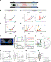
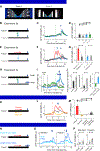
Fig. 1.. Experiments to dissociate value and RPE using virtual reality.

(A) The virtual linear track. (B) State value as a function of position. Red arrow, teleport. (C) Predictions of how state value (left) and TD RPE (right) are modulated by teleport (red curves). (D) Speed manipulation. (E) Predictions. (F) An example scene at the starting position. (G) (top) The time courses of lick rate (gray) and the average across animals (black) (n = 16 mice). (bottom) Locomotor speed (gray) and the average (black). Green, red, and blue horizontal bars represent the time windows used for analysis in Fig. 1H. (H) (top) Impulsive lick (green), anticipatory lick (red), and post-reward lick (blue) rates as a function of days of training. *p < 0.05 (n = 16 mice). Anticipatory lick increased, impulsive lick decreased, and post-reward lick did not change over days of training (r = 0.39,−0.36, 0.04; p = 2.7 × 10⁻⁷, 3.9 × 10⁻⁶, 0.64, respectively, Spearman correlation). (bottom) Locomotor speed. (I) Fiber fluorometry (photometry) experiment. (J) Recording locations in the experimental (green) and GFP control (red) animals (n = 16 and 6 mice, respectively). (K) Average axonal calcium signals (n = 16 mice). A gray horizontal bar depicts a temporal window used to compute Pearson correlations (Ramping R). (L) Ramping Rs. *p < 0.05. (M, N) Signals (M) and ramping Rs (N) from GFP animals (p > 0.05, Wilcoxon signed-rank test for each day, n = 6 mice). See also Fig. S2.

Fig. 2.. Dopamine axon activities in VS are consistent with RPE.

(A) Experiment 1. Long teleport, short teleport, and pause are depicted on the value function. (B) Predictions. T, teleport. P, pause. (C) Average calcium signals aligned by teleport or pause (n = 11 mice). Format as in (B). The trace of the standard condition (black) was aligned by reward onset. (D) Comparisons of normalized peak responses (left) and residuals from the state value prediction (right) (n = 11 mice; Fig. S4A–D). Horizontal bars with filled circle represent significant differences. (E) Experiment 2. Teleports at three positions (T1, T2, T3). (F) Predictions. (G) Average calcium signals (n = 11 mice). Four mice whose scene speed was slightly faster than the rest of animals were excluded in the time course plots but included in other analyses (see Methods). (H) (left) Normalized peaks increase with proximity to the reward (median Test R = 0.45, p = 6.1×10⁻⁵, n = 15 mice). (right) Residuals from the state value prediction (median Test R = 0.20; p = 0.0031, n = 15 mice). (I) Experiment 3. (J) Predictions. (K) Average calcium signals (n = 15 mice). (L) (left) Comparison of average pre-reward responses at [−1 s 0 s] relative to reward. (right) Comparison of regression coefficients. The median of regression coefficients is positive only for the speed of scene movement (p = 6.1 × 10⁻⁵, 0.64, and 0.45, respectively, n = 15 mice). (M) Experiment 4. (N) Predictions. (O) Average calcium signals (n = 5 mice). (P) Comparison of calcium signals before reward.

Fig. 3.. RPE models explain the data better than value models.

(A) Model fitting procedure. Blue curves, GCaMP filters. (B) Fit examples. (top) The data. (middle) Best fit with the RPE model. Thick lines, model prediction. Thin lines, data. (bottom) Best fit with the value model. (C) Comparisons of AICs based on the exponential value function. Filled symbols, p < 0.05 (permutation test). A smaller AIC value indicates a better fit. (D) Difference between the two models in (C). (E) (left) AIC relative to the exponential RPE model. The combined dataset for Experiments 1–3 was used. ${\tau }^{\left(x_0-x\right)}$, exponential discounting; $\beta X=\Sigma \left({\beta }_k{x}^k\right)$, fifth-order polynomial; βX, f’(x) > 0, fifth-order polynomial with the constraint of monotonical increase; Δt to reward, value based on time-to-reward given the current speed. Filled dots indicate significance. (right) Hybrid models. Mixture, (1 − α)V (x) + αδ (x); FD, fractional derivative model. Significance is not shown for the fractional derivative model. (F) The shape of value function (left), RPE (right, dark green), and the predicted calcium signal (right, green) obtained by the RPE model using βX, f’(x) > 0. The peak of the transient RPE at trial start is not shown. (G) The optimal α in the mixture model. (H) The best fit order of derivative (a) in the FD model. See also Figs. S3 and S4.

Fig. 4.. Ramping and teleport responses cannot be explained by a sensory surprise.

(A) The scences on Tracks 1 and 2. (B) Experiment 5a. Arrows, teleports between tracks. (C) Average calcium signals (n = 6 mice). T, teleport. (D) Baseline-subtracted calcium responses. (E) Experiment 5b. Red, forward teleport. Cyan, between-track teleport. (F) Average calcium signals (n = 6 mice). (G) Baseline-subtracted calcium responses. (H) Experiment 5c. Arrows, between-track teleports. Large reward was given in Track 2. (I) Average calcium signals (n = 4 mice). (J) (left) Comparison of anticipatory licking (3/4 mice showed a significant difference, Wilcoxon rank-sum test using trial data). (middle) Comparison of calcium responses (3/4 mice showed a significant difference, unpaired t-test using trial data). (right) Transient changes of calcium responses at teleport (p = 0.006 and 0.021, large to small and small to large, respectively, n = 4 mice, paired t-test). (K) Experiment 6. Arrows, forward (red) and backward (orange) teleports. (L) Average calcium signals (n = 6 mice). (M) Comparisons of calcium responses. Responses to the forward teleports were significantly larger than responses to the backward teleports (p = 0.03, n = 6, Wilcoxon signed rank test) (N) Experiment 7. The reward size was altered across blocks of trials. (O) Average calcium signals (n = 10 mice). (P) Comparison of calcium responses, quantified using the time windows depicted in O (gray bars). (left) Ramp magnitudes. (right) Teleport responses. See also Fig. S4.

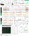
Fig. 5.. Spiking activity of VTA dopamine neurons accounts for the ramping calcium signals.

(A) Experiments. (B) Average firing rates of VTA dopamine neurons (n = 102) in the standard condition. Gray bar, a time window used to quantify ramping in (C). (C) Distribution of ramping Rs. The median (triangle) is positive (p = 0.0001, n = 102 neurons). (D) Ramping slope as a function of ML locations (n = 122). Gray bars, subgroups of neurons used in Fig. 5E, F (Black, n = 16 neurons from 3 mice; dark gray, n = 66 neurons from 4 mice; gray, n = 20 neurons from 3 mice). The median slope was greater than zero in the two medial groups (p = 0.004, 0.009, and 0.39, respectively). Dashed line, type 2 regression fit. (E) Average firing of groups of neurons indicated in D. (F) Calcium signals predicted from spikes. Darkness indicates the groups in D. (G–J) Example neurons. An example neuron that showed positive ramp (G, Ramping R, r = 0.018, p = 0.009), a negative ramp (H, Ramping R, r = −0.0214, p = 0.0001), and no ramp (I, Ramping R, r = 0.005, p = 0.49). (J) A neuron that showed value-like responses (the top row in P). (K) (top) Average spiking activity (n = 88). (bottom) Predicted calcium signals. (L) (top) Average spiking activity (n = 83). (L) (bottom) Predicted calcium signals. (M) Comparisons of goodness-of-fits (AIC). (left) ΔAIC relative to the RPE model based on the exponential value function. Format as Fig. 3E. (right) ΔAIC in hybrid models. (N) The best fit for the mixture model. (O) The best fit order of derivative (a). (P) Single neuron activities. Neurons are sorted by ΔAIC between the value and RPE models (exponential value function) (n = 78 neurons). The area under receiver-operating characteristic curve (auROC) at each time bin was used to quantify firing rate changes from baseline. Arrowheads indicate the time of teleport or pause onset. (Q) Single neuron activities. ΔAIC between the value and RPE models using three different value functions as in Fig. 5M, the best fit order of derivative in the fractional derivative model, and the slope of ramping are shown (n = 78 neurons). (R) (left) Average of the normalized best-fit value functions (n = 78 neurons). (right) The average RPE predicted from the value functions of individual neurons (dark green). Predictied calcium signal (green). See also Fig. S5.

Fig. 6.. Somatic calcium of VTA dopamine neurons and dopamine in VS signal RPEs.

(A) Experiment. (B–D) Average calcium signals in Experiment 1 (B, n = 6 mice), Experiment 2 (n = 6 mice), and Experiment 3 (n = 5 mice). (E) Experiment. (F–H) Average dopamine signals in Experiment 1 (F, n = 9 mice), Experiment 2 (G, n = 10 mice) and Experiment 3 (H, n = 10 mice). See also Fig. S6.

Fig. 7.. Dynamic sensory stimulus indicating reward proximity can cause a dopamine ramp consistent with RPEs.

(A) Delayed-reward task with odor cues. A subset of animals in Fig. 5 were used. (B) Average firing rates (top, n = 67 neurons) and predicted calcium responses (bottom). (C) The standard conditions in the linear track tasks for the same neurons as in (B) (n = 174 sessions from standard and Experiments 1, 3 from n = 67 neurons). (D) Ramping slopes in the delayed reward task (Odor D, slope = −0.06 ± 0.02 spike/s², p = 0.018, n = 67) and the linear track task (average across tasks, slope = 0.10 ± 0.03 spike/s², p = 0.002, n = 67 neurons). (E) Spatial cue manipulations (Experiment 8) (left) patterned, distinct wall patterns were removed. (right) Calcium signals in the standard (black, n = 6 mice) and patterned scene (orange). Arrows, the medians of scene onsets. (F) (left) solid-colored, optic flow was removed by solid-colored stimulus (right). Calcium signals in the standard (black, n = 6 mice) and solid-colored scene (orange). (G) Ramping Rs (p = 0.063 and 0.031 for Experiments 8a and 8b, respectively, n = 6). (H) Moving bar experiment. A reward was delivered when the bar reached a target position (dotted line, illustration purpose only). (I) Experiment 1 with moving bar. Calcium signals aligned by long bar teleport (red), short bar teleport (orange), and pause (yellow) (n = 9 mice). Calcium signals in the standard condition (black) are aligned by reward onset (black dash). (J) Experiment 2 (n = 10 mice). Vertical lines, teleports. (K) Experiment 3 (n = 11 mice). (L) Comparisons of AIC between value and RPE models based on the exponential value function. (M) Difference between the two models. All median ΔAICs except for the standard condition are significantly different from zero (p = [0.20 0.008 0.02 0.04 0.004], n = [9 8 8 9 9]). (N) AICs from variants of models. Format same as Fig. 3E. (O–Q) Average dopamine signals measured using a dopamine sensor. (O) Experiment 1 (n = 8 mice), (P) Experiment 2 (n = 8 mice), and (Q) Experiment 3 (n = 8 mice) using moving bar. See also Fig. S7.

References

1. Akaike H (1973). Information Theory as an Extension of the Maximum Likelihood Principle In Petrov BN and Csaki F (Eds.) Second International Symposium on Information Theory, (Budapest: Akadémiai Kiadó; ), pp. 267–281.
1. Aronov D, and Tank DW (2014). Engagement of Neural Circuits Underlying 2D Spatial Navigation in a Rodent Virtual Reality System. Neuron 84, 442–456. - PMC - PubMed
1. Babayan BM, Uchida N, and Gershman SJ (2018). Belief state representation in the dopamine system. Nature Communications 9, 1891. - PMC - PubMed
1. Bäckman CM, Malik N, Zhang Y, Shan L, Grinberg A, Hoffer BJ, Westphal H, and Tomac AC (2006). Characterization of a mouse strain expressing Cre recombinase from the 3’ untranslated region of the dopamine transporter locus. Genesis 44, 383–390. - PubMed
1. Bayer HM, and Glimcher PW (2005). Midbrain dopamine neurons encode a quantitative reward prediction error signal. Neuron 47, 129–141. - PMC - PubMed
Publication types
LinkOut - more resources