Fractional SIR epidemiological models

Abstract

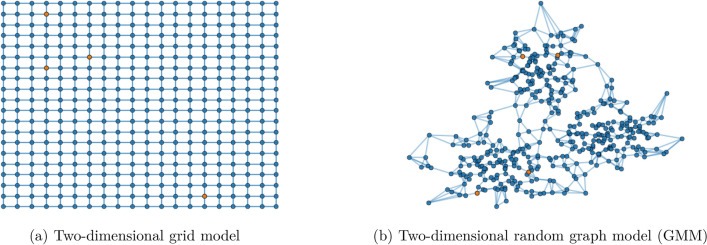
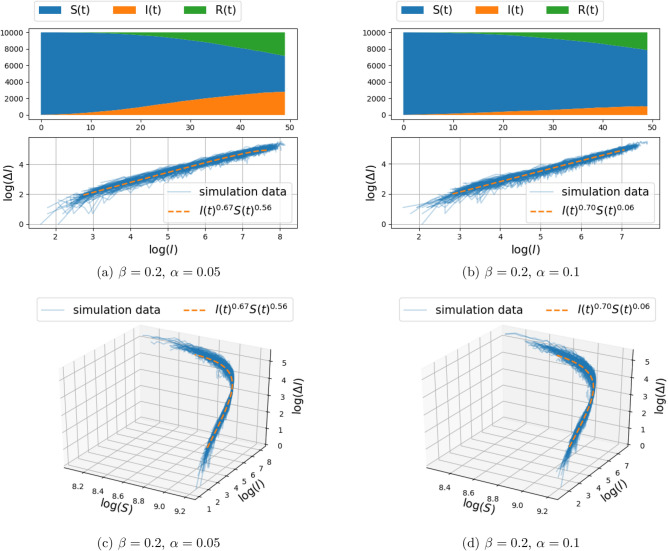
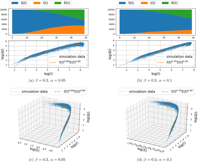
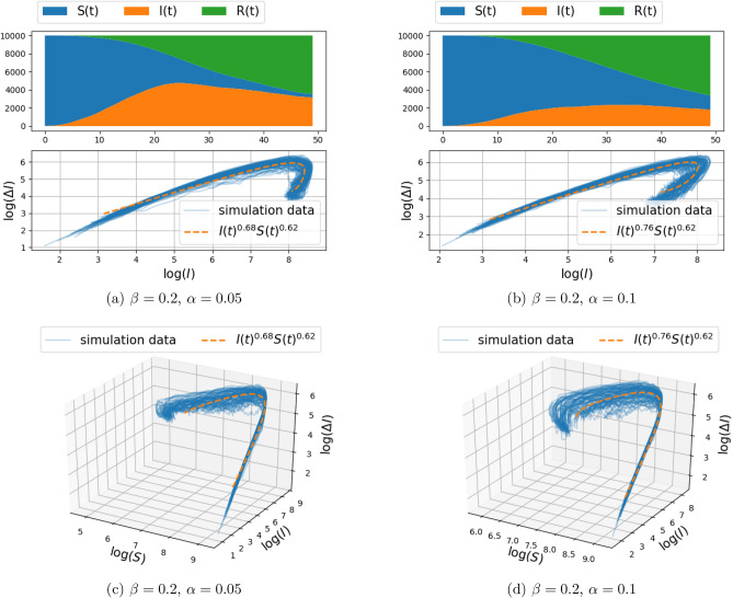
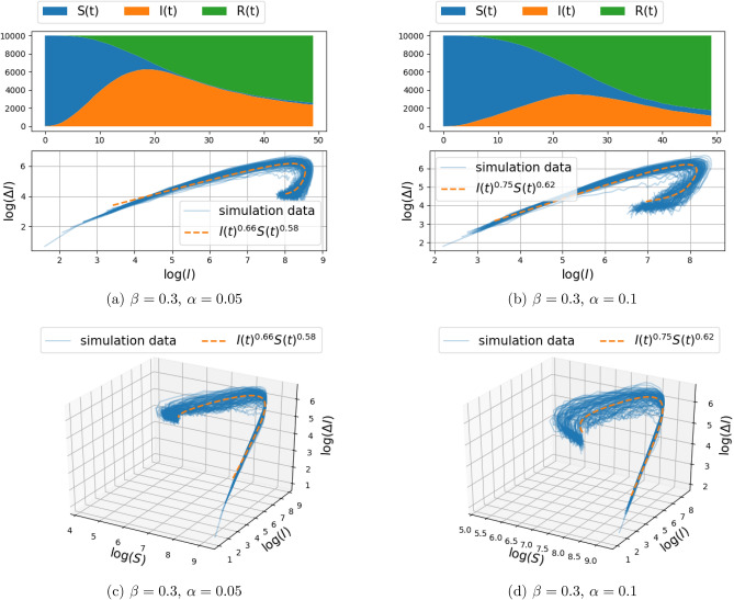
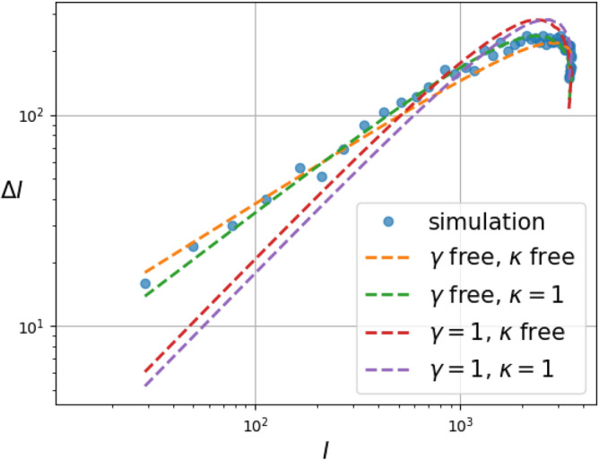
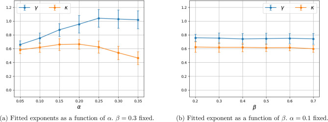
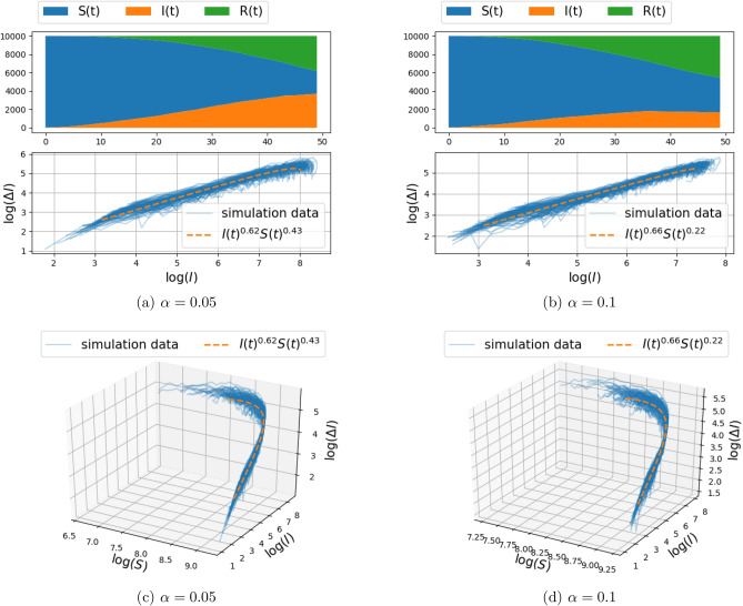
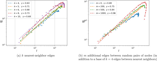
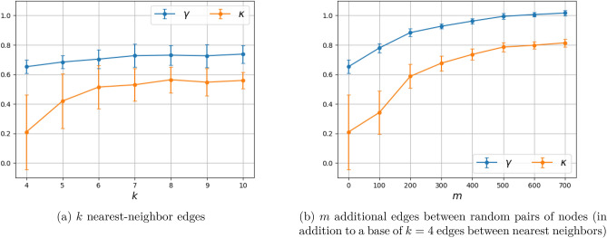
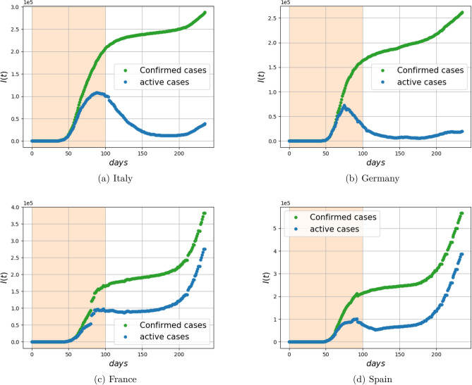
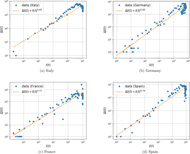
The purpose of this work is to make a case for epidemiological models with fractional exponent in the contribution of sub-populations to the incidence rate. More specifically, we question the standard assumption in the literature on epidemiological models, where the incidence rate dictating propagation of infections is taken to be proportional to the product between the infected and susceptible sub-populations; a model that relies on strong mixing between the two groups and widespread contact between members of the groups. We contend, that contact between infected and susceptible individuals, especially during the early phases of an epidemic, takes place over a (possibly diffused) boundary between the respective sub-populations. As a result, the rate of transmission depends on the product of fractional powers instead. The intuition relies on the fact that infection grows in geographically concentrated cells, in contrast to the standard product model that relies on complete mixing of the susceptible to infected sub-populations. We validate the hypothesis of fractional exponents (1) by numerical simulation for disease propagation in graphs imposing a local structure to allowed disease transmissions and (2) by fitting the model to the JHU CSSE COVID-19 Data for the period Jan-22-20 to April-30-20, for the countries of Italy, Germany, France, and Spain.

Figure 1

Structure of the two graph models considered in this paper. Nodes are connected to their 4 nearest neighbors. The initially infected people are marked in orange.

Figure 2

Spread of infection on a two-dimensional grid, with connection to $k=4$ nearest neighbors (i.e., $d=1$ in Eq. (5)) and transmission rate $\beta =0.2$ (the recovery rate $\alpha$ is fixed to either 0.05 or 0.1). The top panels depict the number of susceptible, infected, and recovered individuals as a function of time over a range of 50 days, for a single realization of the stochastic model described in “Model: probabilistic SIR on a graph”. The center and bottom panel depict $(\mathrm{\Delta }{I}_{\text{trans}}(t),I(t))$ and $(\mathrm{\Delta }{I}_{\text{trans}}(t),I(t),S(t))$ respectively, for 100 Monte-Carlo simulations (with solid blue lines). The fractional model fit is illustrated with orange dashed curve. The fitting procedure maximizes the log-likelihood (9) over the free parameters. The value of the fitted exponents are shown in the legend.

Figure 3

Spread of infection on a two-dimensional grid, with connection to $k=4$ nearest neighbors (i.e., $d=1$ in Eq. (5)) and transmission rate $\beta =0.3$ (the recovery rate $\alpha$ is fixed to either 0.05 or 0.1). The top panels depict the number of susceptible, infected, and recovered individuals as a function of time over a range of 50 days, for a single realization of the stochastic model described in “Model: probabilistic SIR on a graph”. The center and bottom panel depict $(\mathrm{\Delta }{I}_{\text{trans}}(t),I(t))$ and $(\mathrm{\Delta }{I}_{\text{trans}}(t),I(t),S(t))$ respectively, for 100 Monte–Carlo simulations (with solid blue lines). The fractional model fit is illustrated with orange dashed curve. The fitting procedure maximizes the log-likelihood (9) over the free parameters. The value of the fitted exponents are shown in the legend.

Figure 4

Spread of infection on a two-dimensional grid, with connection to $k=8$ nearest neighbors (i.e., $d=2$ in Eq. (5)) and transmission rate $\beta =0.2$ (the recovery rate $\alpha$ is fixed to either 0.05 or 0.1). The top panels depict the number of susceptible, infected, and recovered individuals as a function of time over a range of 50 days, for a single realization of the stochastic model described in “Model: probabilistic SIR on a graph”. The center and bottom panel depict $(\mathrm{\Delta }{I}_{\text{trans}}(t),I(t))$ and $(\mathrm{\Delta }{I}_{\text{trans}}(t),I(t),S(t))$ respectively, for 100 Monte-Carlo simulations (with solid blue lines). The fractional model fit is illustrated with orange dashed curve. The fitting procedure maximizes the log-likelihood (9) over the free parameters. The value of the fitted exponents are shown in the legend.

Figure 5

Spread of infection on a two-dimensional grid, with connection to $k=8$ nearest neighbors (i.e., $d=2$ in Eq. (5)) and transmission rate $\beta =0.3$ (the recovery rate $\alpha$ is fixed to either 0.05 or 0.1). The top panels depict the number of susceptible, infected, and recovered individuals as a function of time over a range of 50 days, for a single realization of the stochastic model described in “Model: probabilistic SIR on a graph”. The center and bottom panel depict $(\mathrm{\Delta }{I}_{\text{trans}}(t),I(t))$ and $(\mathrm{\Delta }{I}_{\text{trans}}(t),I(t),S(t))$ respectively, for 100 Monte-Carlo simulations (with solid blue lines). The fractional model fit is illustrated with orange dashed curve. The fitting procedure maximizes the log-likelihood (9) over the free parameters. The value of the fitted exponents are shown in the legend.

Figure 6

Comparison of four fSIR models with free and partially specified choice of exponents (with the SIR model corresponding to $\gamma =1$ and $\kappa =1$) based on simulation data obtained from two-dimensional grid model with infection parameter $\alpha =0.05$ and $\beta =0.3$. The AIC and maximum likelihood scores for these models are reported in Table 3.

Figure 7

Dependence of the fitted exponents $\gamma$ and $\kappa$ on the model parameters $\alpha$ and $\beta$ for the two-dimensional grid model with $k=4$ nearest neighbors. (Mean and error bars for standard deviation are based on 100 Monte Carlo simulations).

Figure 8

Spread of infection on a mixture of Gaussian random graph model for transmission rate $\beta =0.3$ (the recovery rate $\alpha =0.05$ or $\alpha =0.1$).The top panels depict the number of susceptible, infected, and recovered individuals as a function of time over a range of 50 days, for a single realization of the stochastic model described in “Model: probabilistic SIR on a graph”. The center and bottom panel depict $(\mathrm{\Delta }{I}_{\text{trans}}(t),I(t))$ and $(\mathrm{\Delta }{I}_{\text{trans}}(t),I(t),S(t))$ respectively, for 100 Monte–Carlo simulations (with solid blue lines). The fractional model fit is illustrated with orange dashed curve. The fitting procedure maximizes the log-likelihood (9) over the free parameters. The value of the fitted exponents are shown in the caption.

Figure 9

Dependence of the fitted exponent $\gamma$ on graph connectivity for the mixture of Gaussian random graph model. The infection parameters $\alpha =0.1$ and $\beta =0.3$ are fixed. The network parameters, the number of nearest neighbors k and the number of random additional edges m vary. A single realization is displayed for each choice of network parameters.

Figure 10

Dependence of the fitted exponents $\gamma$ and $\kappa$ on graph connectivity for the mixture of Gaussian random graph model. The infection parameters $\alpha =0.1$ and $\beta =0.3$ are fixed. The network parameters, the number of nearest neighbors k and the number of random additional edges m vary. (Mean and error bars for standard deviation are based on 100 Monte Carlo simulations).

Figure 11

Number of confirmed and active cases in four different countries during the period 01/22/2020 to 09/13/2020. The shaded area is the time period where the fractional model is used to fit the data in Fig. 12. The number of active cases is computed by subtracting the total deaths and recovered from total confirmed cases.

Figure 12

Relationship between infection growth due to transmission $\mathrm{\Delta }{I}_{\text{trans}}(t)$ and the number of infected individuals I(t) (active cases) with COVID-19 in four different countries. The data belongs to the first 100 days of the infection starting from 01/22/2020.

References

-
- Bauer F, Castillo-Chavez C, Feng Z. Mathematical Models in Epidemiology. Berlin: Springer; 2019.
- Bjørnstad ON, Shea K, Krzywinski M, Altman N. Modeling infectious epidemics. Nat. Methods. 2020;20:20. - PubMed
- Capasso V. Mathematical Structures of Epidemic Systems. Berlin: Springer; 2008.
Publication types
MeSH terms
Grants and funding
LinkOut - more resources
Full Text Sources
Medical
Research Materials
Miscellaneous