Circadian Rhythms of Early Afterdepolarizations and Ventricular Arrhythmias in a Cardiomyocyte Model

Abstract

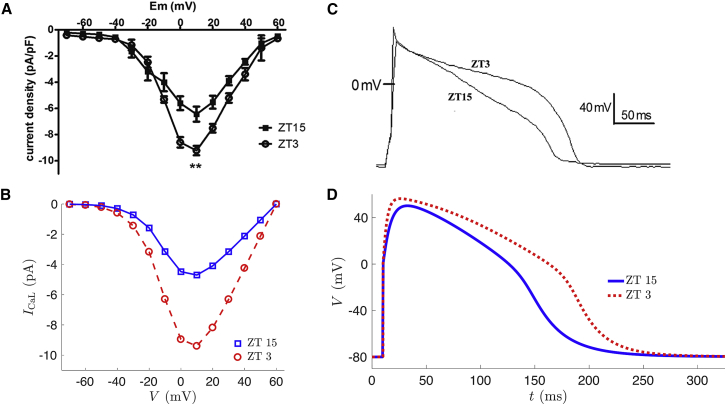
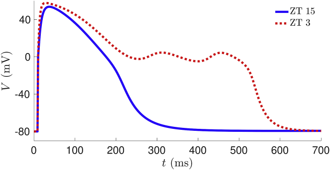
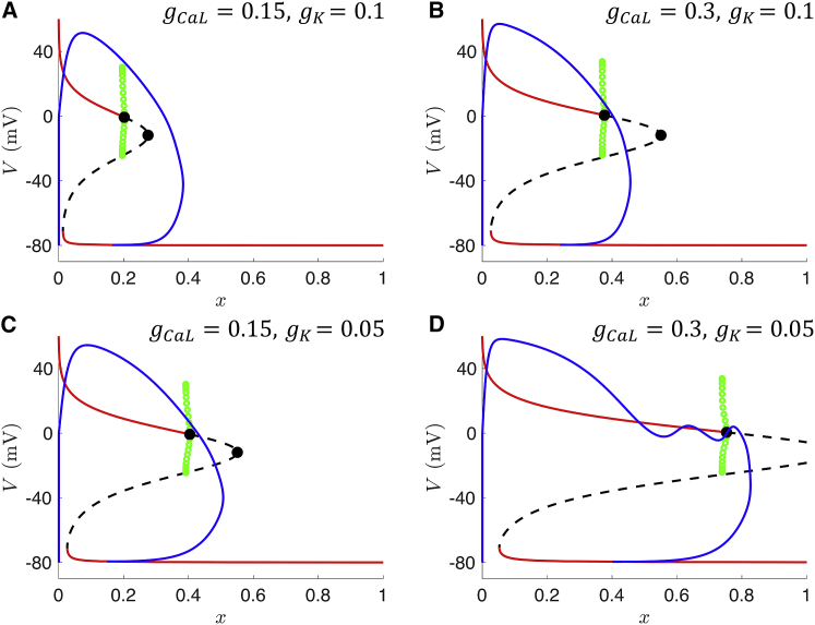
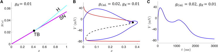
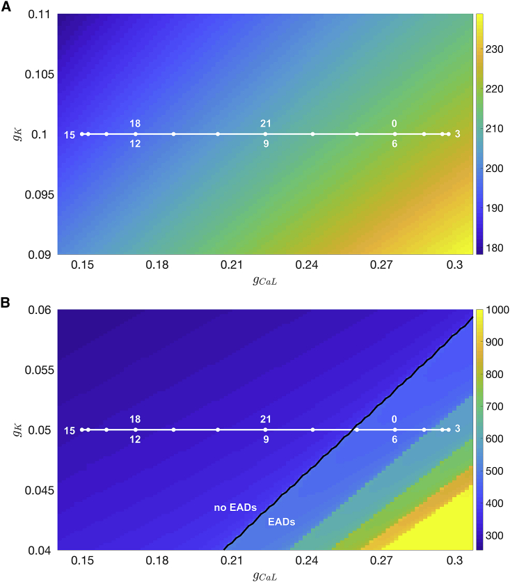
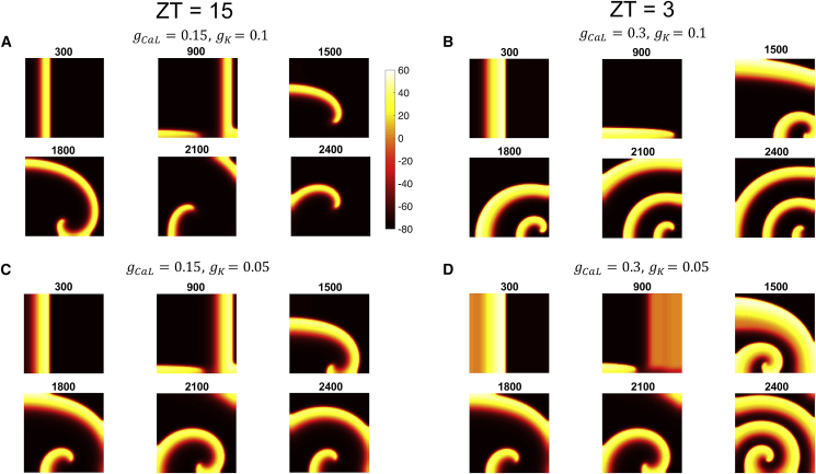
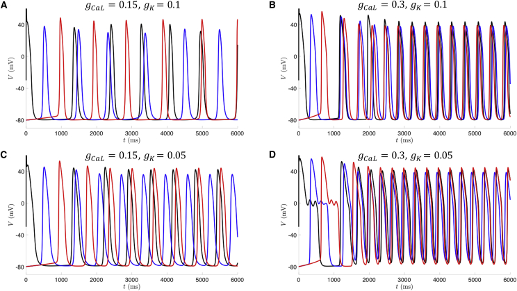
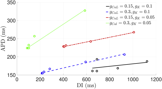
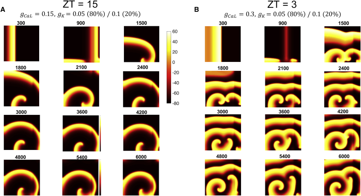
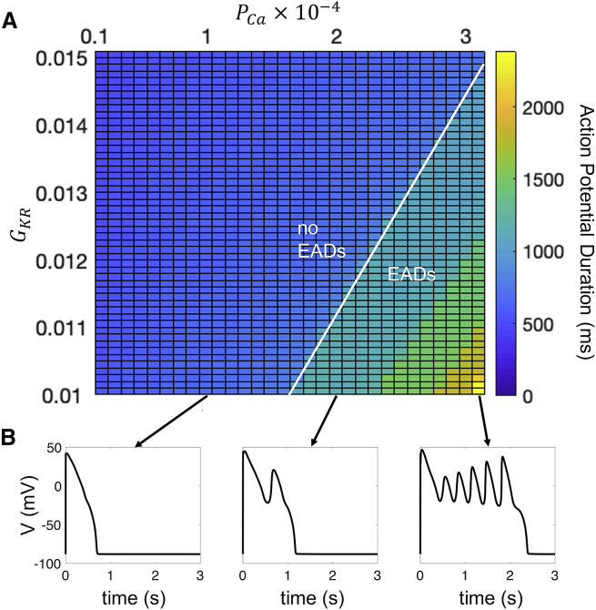
Sudden cardiac arrest is a malfunction of the heart's electrical system, typically caused by ventricular arrhythmias, that can lead to sudden cardiac death (SCD) within minutes. Epidemiological studies have shown that SCD and ventricular arrhythmias are more likely to occur in the morning than in the evening, and laboratory studies indicate that these daily rhythms in adverse cardiovascular events are at least partially under the control of the endogenous circadian timekeeping system. However, the biophysical mechanisms linking molecular circadian clocks to cardiac arrhythmogenesis are not fully understood. Recent experiments have shown that L-type calcium channels exhibit circadian rhythms in both expression and function in guinea pig ventricular cardiomyocytes. We developed an electrophysiological model of these cells to simulate the effect of circadian variation in L-type calcium conductance. In our simulations, we found that there is a circadian pattern in the occurrence of early afterdepolarizations (EADs), which are abnormal depolarizations during the repolarization phase of a cardiac action potential that can trigger fatal ventricular arrhythmias. Specifically, the model produces EADs in the morning, but not at other times of day. We show that the model exhibits a codimension-2 Takens-Bogdanov bifurcation that serves as an organizing center for different types of EAD dynamics. We also simulated a two-dimensional spatial version of this model across a circadian cycle. We found that there is a circadian pattern in the breakup of spiral waves, which represents ventricular fibrillation in cardiac tissue. Specifically, the model produces spiral wave breakup in the morning, but not in the evening. Our computational study is the first, to our knowledge, to propose a link between circadian rhythms and EAD formation and suggests that the efficacy of drugs targeting EAD-mediated arrhythmias may depend on the time of day that they are administered.

Figure 1

Fitting model parameters to voltage and current-clamp data from guinea pig cardiomyocytes. (a) Voltage-clamp data of L-type calcium current from (16) are shown. (b) Simulated voltage-clamp experiment with g_CaL = 0.3 mS/cm² (dashed red line and open circles) and g_CaL = 0.15 mS/cm² (solid blue line and open squares) is shown for g_K = 0.1 mS/cm². (c) Current-clamp recording of action potentials in guinea pig cardiomyocytes from (16) is shown. (d) Simulated current-clamp experiment with g_CaL = 0.3 mS/cm² (dashed red line) and g_CaL = 0.15 mS/cm² (solid blue line) is shown for g_K = 0.1 mS/cm². To see this figure in color, go online.

Figure 2

Model exhibits early afterdepolarizations for high g_CaL and low g_K. Voltage trajectories from simulated current-clamp experiments with g_CaL = 0.3 mS/cm² (dashed red line) and g_CaL = 0.15 mS/cm² (solid blue line) are shown for g_K = 0.05 mS/cm². To see this figure in color, go online.

Figure 3

Bifurcation diagrams with bifurcation parameter x for various values of g_CaL and g_K. Trajectories from the full system (solid blue lines) are projected onto the x-V plane and overlayed with steady states of the fast subsystem (solid red lines are stable, dashed black lines are unstable), along with bifurcation points (solid black dots) and unstable periodic orbits (open green circles) emanating from the subcritical Hopf bifurcation. (a) Normal APs for g_CaL = 0.15 mS/cm² and g_K = 0.1 mS/cm² are shown. (b) Increased APD, but not EADs, with increased g_CaL is shown. (c) Increased APD, but not EADs, with reduced g_K is shown. (d) EADs with increased g_CaL and reduced g_K are shown. To see this figure in color, go online.

Figure 4

EAD generation via a different dynamical mechanism near the Takens-Bogdanov (TB) bifurcation point. (a) Two-parameter bifurcation diagram showing the location of Hopf bifurcations (H, cyan curve) and saddle-node bifurcations (SN, magenta curve) is given for bifurcation parameters g_CaL and x, with g_K = 0.01 mS/cm². The Hopf and SN curves coalesce at a codimension-2 TB bifurcation (solid black dot). (b) Trajectory exhibiting an EAD (solid blue line) from the full system projected onto the x-V plane and overlayed with steady states of the fast subsystem (solid red lines are stable, dashed black lines are unstable), along with the saddle-node bifurcation point (solid black dot), is shown for maximal conductance parameters (g_CaL = 0.02 mS/cm², g_K = 0.01 mS/cm²) chosen near the TB bifurcation point shown in (a). (c) Voltage time course of the EAD trajectory shown in (b) is given. To see this figure in color, go online.

Figure 5

Action potential durations and EADs over a circadian cycle. Colorbar indicates APD (in ms), solid white dots are hourly ZT markers, and black lines separate regions of parameter space with and without EADs. (a) Circadian variation of g_CaL (Eq. 8) with g_K = 0.1 mS/cm² does not result in EADs. (b) Circadian variation of g_CaL with reduced g_K = 0.05 mS/cm² is shown. EADs occur between ZT 23 and ZT 7. To see this figure in color, go online.

Figure 6

Spiral waves in a 2-D domain. Color bar indicates membrane voltage (mV) at snapshots of t = 300, 900, 1200, 1500, 1800, 2100, and 2400 ms for simulations of Eq. 9 on a 128 × 128 grid under an S1-S2 cross-field stimulation protocol. (a) Parameters corresponding to ZT 15 (g_CaL = 0.1 mS/cm²) with g_K = 0.1 mS/cm² are shown. (b) Parameters corresponding to ZT 3 (g_CaL = 0.3 mS/cm²) with g_K = 0.1 mS/cm² are shown. (c) Parameters corresponding to ZT 15 (g_CaL = 0.1 mS/cm²) with reduced g_K = 0.05 mS/cm² are shown. (d) Parameters corresponding to ZT 3 (g_CaL = 0.3 mS/cm²) with reduced g_K = 0.05 mS/cm², which produce EADs in the isolated single-cell model as shown in Fig. 3D, are shown. To see this figure in color, go online.

Figure 7

Voltage trajectories for three locations in the 2-D spatial model. Leftmost (black), center (blue), and rightmost (red) grid points for the middle row of the 128 × 128 domain shown in Fig. 6 are given. (a) Parameters corresponding to ZT 15 (g_CaL = 0.1 mS/cm²) with g_K = 0.1 mS/cm² are shown. (b) Parameters corresponding to ZT 3 (g_CaL = 0.3 mS/cm²) with g_K = 0.1 mS/cm² are shown. (c) Parameters corresponding to ZT 15 (g_CaL = 0.1 mS/cm²) with reduced g_K = 0.05 mS/cm² are shown. (d) Parameters corresponding to ZT 3 (g_CaL = 0.3 mS/cm²) with reduced g_K = 0.05 mS/cm² are shown. To see this figure in color, go online.

Figure 8

APD restitution curves from the 2-D spatial model. APD and diastolic interval (DI) were calculated for the leftmost (black) voltage trajectories shown in Fig. 7. Open circles denote (DI, APD) values from each of the four simulations. Linear fits to the data points for the simulations shown in Fig. 7A (solid black), Fig. 7B (dashed blue), Fig. 7C (dashed-dotted red), and Fig. 7D (dotted green) are shown. To see this figure in color, go online.

Figure 9

Spiral wave breakup in a 2-D domain. The same simulation and stimulation protocol as Fig. 6 are used but with heterogeneity in potassium conductance across the domain; g_K = 0.05 mS/cm² for the leftmost 80% of the domain and g_K = 0.1 mS/cm² for the rightmost 20%. (a) Single spiral wave for parameters corresponding to ZT 15 (g_CaL = 0.15 mS/cm²) is shown. (b) Breakup into multiple spiral waves for parameters corresponding to ZT 3 (g_CaL = 0.3 mS/cm²) is shown. To see this figure in color, go online.

Figure 10

EADs in the ORd model. (a) Action potential duration is shown for a range of P_Ca- and G_Kr-values. For (P_Ca, G_KR) parameter combinations below and to the right of the white line, the ORd model exhibits EADs. (b) Voltage traces for simulations with increasing P_Ca-values and G_KR = 0.01 are shown. With P_Ca = 1 × 10⁻⁴, the model does not produce EADs (left panel). With P_Ca = 2 × 10⁻⁴, the model produces a single EAD (middle panel). With P_Ca = 3 × 10⁻⁴, the model produces multiple EADs (right panel). To see this figure in color, go online.