Robust and Scalable Learning of Complex Intrinsic Dataset Geometry via ElPiGraph

Abstract

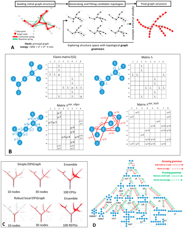
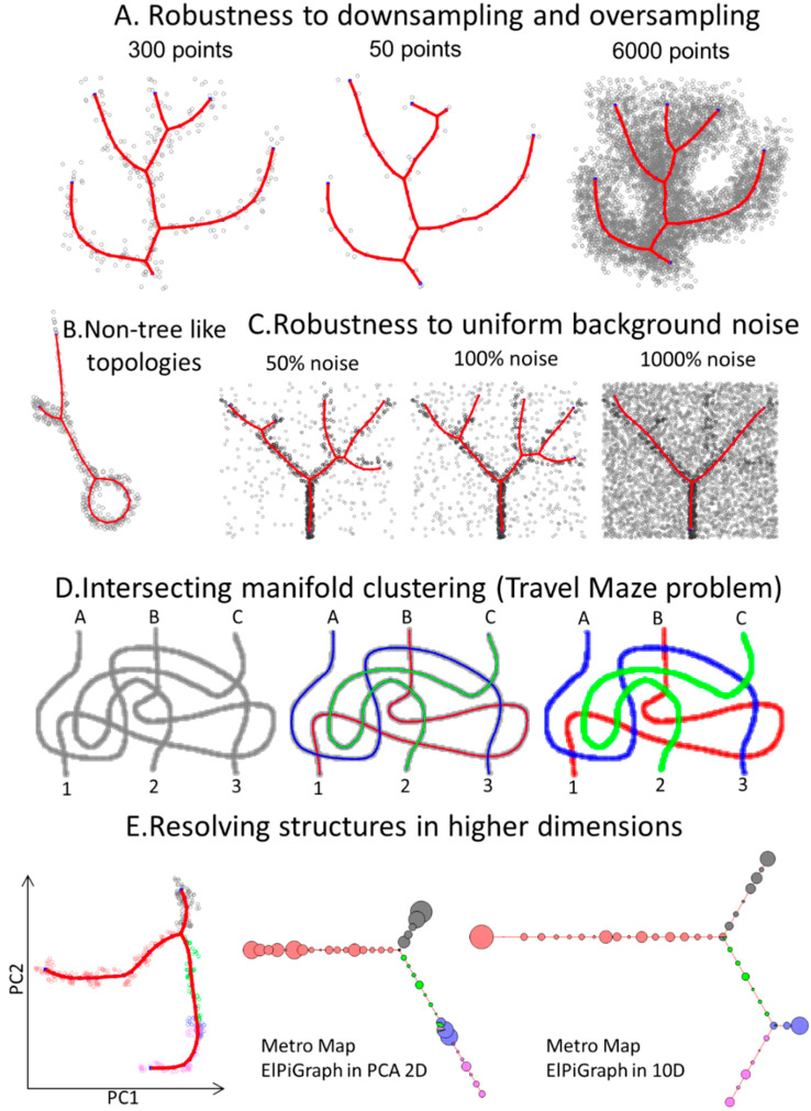
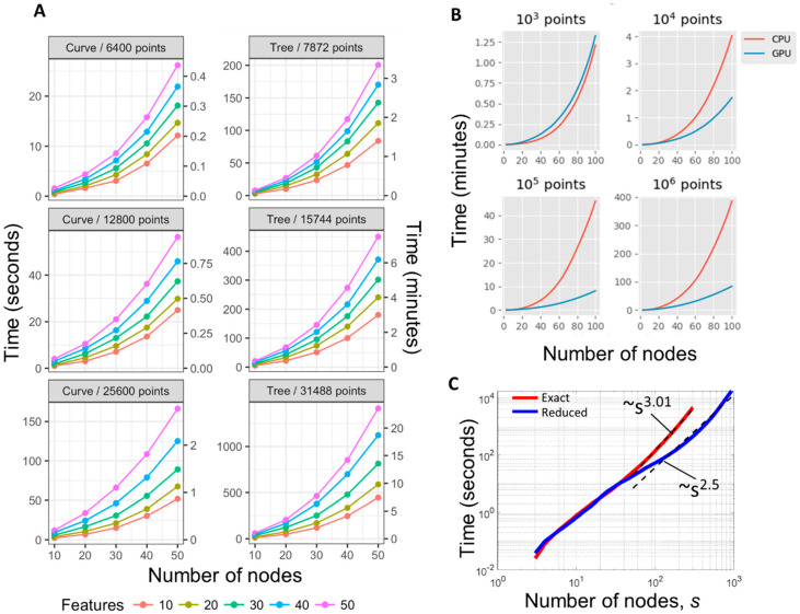
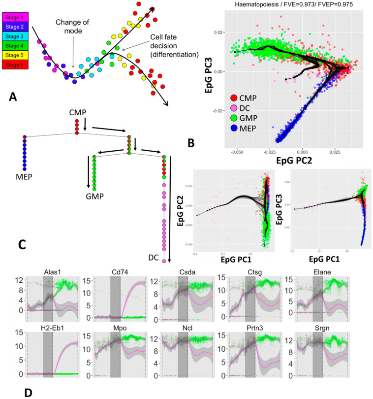
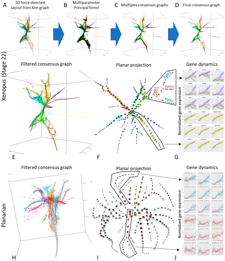
Multidimensional datapoint clouds representing large datasets are frequently characterized by non-trivial low-dimensional geometry and topology which can be recovered by unsupervised machine learning approaches, in particular, by principal graphs. Principal graphs approximate the multivariate data by a graph injected into the data space with some constraints imposed on the node mapping. Here we present ElPiGraph, a scalable and robust method for constructing principal graphs. ElPiGraph exploits and further develops the concept of elastic energy, the topological graph grammar approach, and a gradient descent-like optimization of the graph topology. The method is able to withstand high levels of noise and is capable of approximating data point clouds via principal graph ensembles. This strategy can be used to estimate the statistical significance of complex data features and to summarize them into a single consensus principal graph. ElPiGraph deals efficiently with large datasets in various fields such as biology, where it can be used for example with single-cell transcriptomic or epigenomic datasets to infer gene expression dynamics and recover differentiation landscapes.

Keywords: data approximation; principal graphs; principal trees; software; topological grammars.

Figure 1

Basic principles and examples of ElPiGraph usage. (A) Schematic workflow of the ElPiGraph method. Left, construction of the elastic graph starts by defining the initial graph topology and embedding it into the data space. The graph structure is fit to the data, using minimization of the mean square error regularized by the elastic energy. The elastic energy includes a term reflecting the overall stretching of the graph (symbolically shown as contractive red springs) and a term reflecting the overall bending of the graph branches and the harmonicity of branching points (shown as repulsive green springs). Middle, ElPiGraph explores a large region of the structural space by exhaustively applying a set of graph rewriting rules (graph grammars) and selecting, at each step, the structure leading to the minimum overall energy of the graph embedding. (B) Example of elastic matrix for a simple graph and transforming this matrix into several parts used for optimization (see details in the Methods). (C) Left and middle, illustration of the robust local workflow of ElPiGraph, which makes it possible to deal with the presence of noise. In the global version, the graph structure is fit to all data points at the same time, while in the local version, the structure is fit to the points in the local graph neighborhood, which expands as the graph grows. Right, an illustration of principal graph ensemble approach: 100 elastic principle graphs are superimposed, each constructed on a fraction of data points randomly sampled at each execution. (D) Application of a set of graph grammar rules to generate a set of tree topologies with up to seven nodes.

Figure 2

Synthetic examples showing features of ElPiGraph. (A) ElPiGraph is robust with respect to downsampling and oversampling of a dataset. Here, a reference branching dataset [32] is downsampled to 50 points (middle) or oversampled by sampling 20 points randomly placed around each point of the original dataset. More systematic study of the down/over-sampling effect on robustness of the principal graph is shown in Supplementary Figure S2. (B) ElPiGraph is able to capture non-tree like topologies. Here, the standard set of principal tree graph grammars was applied to a graph initialized by four nodes connected to a ring. (C) ElPiGraph is robust to large amounts of uniformly distributed background noise. Here, the initial dataset from Figure 1 is shown as black points, and the uniformly distributed noisy points are shown as grey points. ElPiGraph is blindly applied to the union of black and grey points. (D) ElPiGraph is able to solve the problem of learning intersecting manifolds. On the left, a toy dataset of three uniformly sampled curves intersecting in many points is shown. ElPiGraph starts by learning a principal curve using the local version several times, each time on a complete dataset. However, for each iteration, ElPiGraph is initialized by a pair of neighboring points not belonging to points already captured by a principal curve. The fitted curves are shown in the middle of the point distribution by using different colors, and the clustering of the dataset based on curve approximation is shown on the right. (E) Approximating a synthetic ten-dimensional dataset with known branch structure (with different colors indicating different branches), where one of the branches (blue one) extrude into higher dimensions and collapses with other branches when projected in 2D by principal component analysis (left). Middle, being applied in the space of two first principal components, ElPiGraph does not recover the branch, while it is captured when the ElPiGraph is applied in the complete 10-dimensional dataset (right). In both cases, the principal tree is visualized using metro map layout [21], and a pie chart associated to each node of the graph indicates the percentage of points belonging to the different populations. The size of the pie chart indicates the number of points associated with each node.

Figure 3

Computational performance of ElPiGraph. (A) Time required to build principal curves and trees (y-axis) with a different number of nodes (x-axis) using the default parameters across synthetic datasets containing different numbers of points having a different number of dimensions (color scale), using single CPU. (B) Demonstrating computational advantages of using a combination of GPU and CPU in ElPiGraph computations. Starting from 10k data points, using GPU becomes advantageous. The computational experiment was done using Google Colab environment. (C) Empirical performance scaling of ElPiGraph on a 12k data points in 5D example. The exact ElPiGraph algorithm scales as polynome of degree 3, while the approximate reduced algorithm with a limitation on the number of tested candidate structures scales as s^2.5 in the s = 50…1000 range, where s is the number of nodes in the principal graph.

Figure 4

Quantification of branching cellular trajectories from single cell scRNASeq data using ElPiGraph. (A) Diagrammatic representation of the concept behind branching cellular trajectories and biological pseudotime in an arbitrary 2D space associated with gene expression: as cells progress from Stage 1 they differentiate (Stages 2 and 3) and branch (Stage 4) into two different subpopulations (Stages 5 and 6). Local distances between the cells indicate epigenetic similarity. Note how embedding a tree into the data allow recovering genetic changes associated with cell progression into the two differentiated states. (B) Application of ElPiGraph to scRNA-Seq data [59]. Each point indicates a cell and is color-coded using the cellular phenotype specified in the original paper. One hundred bootstrapped trees are represented (in black), along with the tree fitted on all the data (black nodes and edges). Projection on ElPiGraph principal components 2 and 3 is shown enlarged as the most informative. The fraction of variance of the original data explained by the projection on the nodes (FVE) and on the edges (FVEP) is reported on top of the plot. (C) Diagrammatic representation of the distribution of cells across the branches of the tree reconstructed by ElPiGraph with the same color scheme as in panel B. Pie charts indicate the distribution of populations associated with each node. The black arrows highlight a particular cell fate decision trajectory from CMP to GMP and DC. (D) Single-cell dynamics of gene expression along the path from the root of the tree (at the top of panel C) to the branch corresponding to DC commitment and GMP commitment. The expression profiles have been fitted by a LOESS smoother, colored according to the majority cell type in the branch, with a 95% confidence interval (in grey). The vertical grey area represents a 95% confidence interval obtained by projecting the relevant branching points of the resampled tree showed in panel B on the path of the principal graph.

Figure 5

Using ElPiGraph to approximate complex datasets describing developing embryos (xenopus) or adult organisms (planarian). (A) A kNN graph constructed using the gene expression of 7936 cells of Stage 22 Xenopus embryo has been projected on a 3D space using a force directed layout. The color in this and the related panels indicate the population assigned to the cells by the source publication. (B) The coordinates of the points in panel A have been used to fit 1280 principal trees with different parameters, hence obtaining a principal forest. (C) The principal forest shown in panel B has been used to produce 10 consensus graphs (one for each parameter set). (D) A final consensus graph has been produced using the consensus graphs shown in panel C. (E) A final principal graph has been obtained by applying standard grammar operations to the consensus graph shown in panel D. (F) The associations of the different cell types to the nodes of the consensus graph shown in panel E is reported on a plane with a pie chart for each node. Note the complexity of the graph and the predominance of different cell types in different branches, as indicated the predominance of one or few colors. (G) The dynamics of notable genes had been derived by deriving a pseudotime for a branching structure (top) and a linear structure (bottom) present in the principal graph of panel E (see black polygons). Each point represents the gene expression of a cell and their color indicate either their associated path (top) of the cell type (bottom). The gene expression profiles have been fitted with a LOESS smoother which include a 95% confidence interval. In the top panel the smoother has been colored to highlight the different paths, with the color indicated in the text of panel F. (H–J) The same approach described by panels A–G has been used to study the single-cell transcriptome of planarians. In panel J, the color of the smoother indicates the predominant cell type on the path. Interactive versions of key panels are available at https://sysbio-curie.github.io/elpigraph/.

References

1. Roux B.L., Rouanet H. Geometric Data Analysis: From Correspondence Analysis to Structured Data Analysis. Springer; Dordrecht, The Netherlands: 2005.
1. Gorban A., Kégl B., Wunch D., Zinovyev A. Principal Manifolds for Data Visualisation and Dimension Reduction. Springer; Berlin/Heidelberg, Germany: 2008.
1. Carlsson G. Topology and data. Bull. Am. Math. Soc. 2009;46:255–308. doi: 10.1090/S0273-0979-09-01249-X. - DOI
1. Nielsen F. An elementary introduction to information geometry. arXiv Prepr. 20181808.08271 - PMC - PubMed
1. Camastra F., Staiano A. Intrinsic dimension estimation: Advances and open problems. Inf. Sci. 2016;328:26–41. doi: 10.1016/j.ins.2015.08.029. - DOI
LinkOut - more resources