Genetic interaction mapping informs integrative structure determination of protein complexes

Abstract

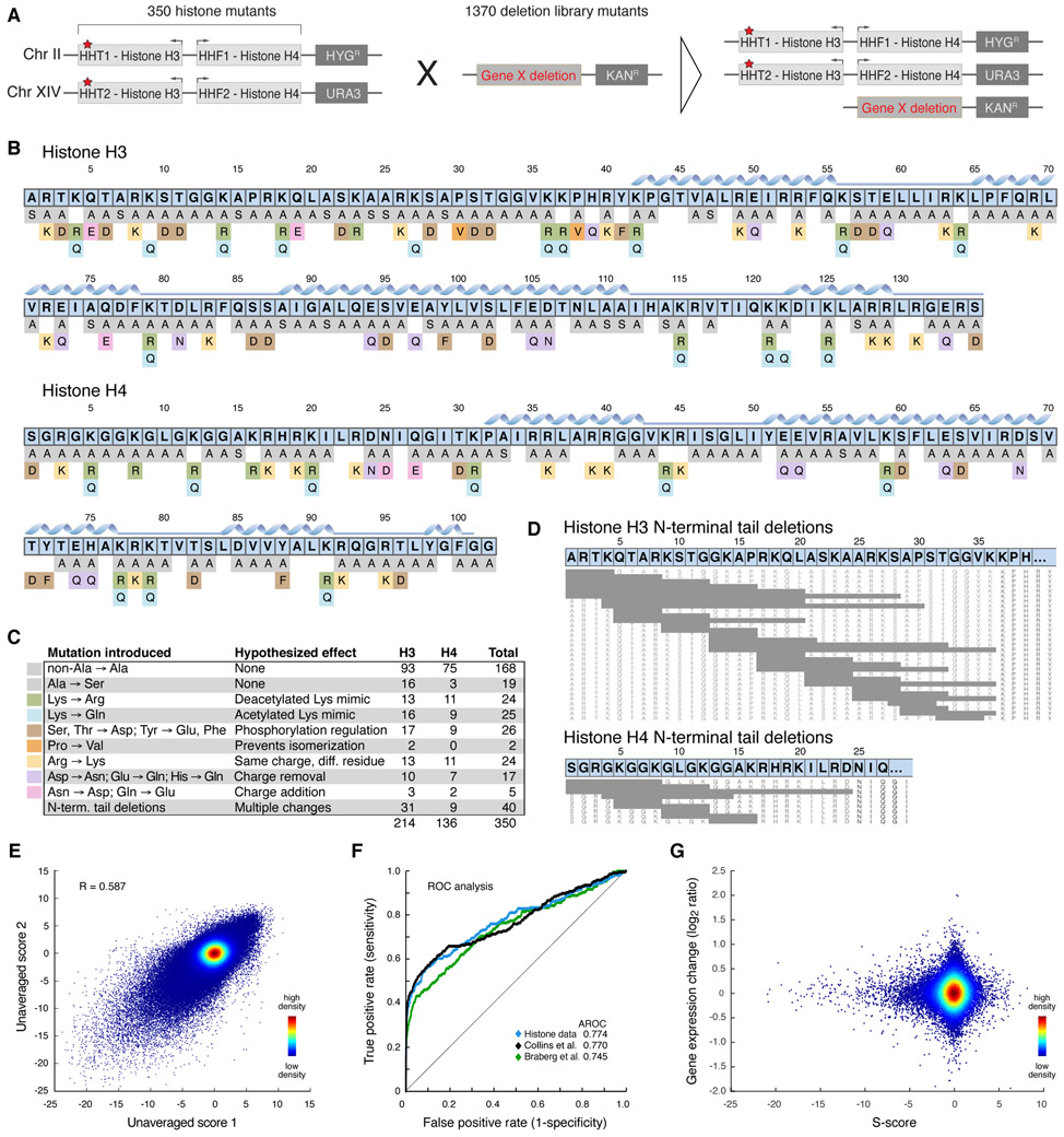
Determining structures of protein complexes is crucial for understanding cellular functions. Here, we describe an integrative structure determination approach that relies on in vivo measurements of genetic interactions. We construct phenotypic profiles for point mutations crossed against gene deletions or exposed to environmental perturbations, followed by converting similarities between two profiles into an upper bound on the distance between the mutated residues. We determine the structure of the yeast histone H3-H4 complex based on ~500,000 genetic interactions of 350 mutants. We then apply the method to subunits Rpb1-Rpb2 of yeast RNA polymerase II and subunits RpoB-RpoC of bacterial RNA polymerase. The accuracy is comparable to that based on chemical cross-links; using restraints from both genetic interactions and cross-links further improves model accuracy and precision. The approach provides an efficient means to augment integrative structure determination with in vivo observations.

Fig. 1.. Building spatial restraints from pairwise genetic perturbations.

(A) Genetic interactions arise when the combined fitness defect of a double mutant deviates from the expected multiplicative growth defect of the two single mutants. (B) The generation of a pE-MAP relies on a collection of point mutations, which is constructed by systematic mutagenesis of genes that encode the subunits of a macromolecular assembly (mutations labeled 1-4). The point mutant strains are then crossed against a library of gene deletions, followed by fitness measurement and subsequent calculation of genetic interaction scores to obtain the phenotypic profiles. (C) An example subset of a pE-MAP of point mutants crossed against a library of gene deletions. (D) Each pairwise combination of phenotypic profiles is transformed into a single MIC value that reflects the similarity between the two profiles. The MIC values are translated into spatial restrains for integrative modeling. (E) The MIC values and other input information are used for integrative structure modeling. An ensemble of structures that satisfy the input information is obtained.

Fig. 2.. Genetic interrogation of histones H3 and H4 at a residue-level resolution.

(A) Each histone mutant strain was modified at both native loci (HHT1 & HHT2 for H3 or HHF1 & HHF2 for H4, red stars) and crossed against a library of 1370 different deletion mutants (or hypomorphic alleles for essential genes). (B) Schematic of the histone point mutants analyzed in this study (Table S1). Secondary structure elements are indicated as ribbons above the amino acid sequence. The mutations are color-coded according to the mutation introduced (Fig. 2C). Mutations resulting in inviable strains or strains too sick for genetic analysis are shown in Fig. S1. (C) Table of histone mutant categories and their hypothesized effects (color coding as in Fig. 2B). (D) Overview of viable H3 and H4 tail deletion mutants amenable to pE-MAP analysis. The amino acid sequences of the wt alleles are shown on top (residues 1-39 of histone H3 and 1-27 of histone H4). Grey bars signify the deleted residues in H3 and H4. (E) Reproducibility of histone pE-MAP S-scores between biological replicates. Plotted are all S-score pairs among the biological replicas, which include triplicate measurements for 346 histone alleles and duplicates of 4 alleles (H4E73Q, H4H18A, H4121A and H4K44Q). (F) ROC curves showing the power to predict physical interactions between pairs of proteins from this pE-MAP (blue) as well as previously published pE-MAP (green, (15)) and E-MAP (black, (29)) data. (G) Relationship between gene expression (log₂ fold-change over wt) and S-scores of 29 H3 and H4 alleles (Table S2). Data from all 1,256 deletion library mutants that were measured in both RNAseq expression and pE-MAP analysis are plotted.

Fig. 3.. The genetic interaction landscape of histones H3 and H4.

(A) Hierarchically clustered pE-MAP of 350 histone H3 and H4 alleles screened against a library of 1,370 deletion mutants or hypomorphic alleles. The pE-MAP consists of more than 479,000 genetic interactions. Positive- (suppressive/epistatic) and negative (synthetic sick) genetic interactions are colored in yellow or blue, respectively. Examples of histone alleles with similar genetic interaction profiles are highlighted on the right side in context of the nucleosome structure. The nucleosome structure is modified from PDB 1ID3 (Data S2), with H3 in purple, H4 in green, and mutated or deleted residues highlighted in red. N-terminal tail residues of H3 and H4 not included in 1ID3 are visualized as strings on the periphery. (B) Examples of genetic interaction profiles of gene clusters belonging to known protein complexes or biological pathways are highlighted and their genetic interaction profiles enlarged from Fig. 3A. DDR - DNA damage/repair, UPP - ubiquitin proteasome pathway.

Fig. 4.. Generation of the scoring function

(A) Relationship between pairwise distances and MIC values. The solid grey line represents the logarithmic decay fit to the upper distance bounds (Methods, Eq. 1). The background color gradient reflects how the data likelihood depends on MIC value and distance. (B) -Log of the data likelihood as a function of distance for different MIC values (Methods).

Fig. 5.. Description of the integrative modeling workflow.

The four stages include: (1) gathering all available experimental data and prior information; (2) translating all information into a representation of the assembly components and a scoring function for ranking alternative assembly structures; (3) sampling structural models; and (4) validating the model. In this example, the representation of the components of a complex is based on comparative models of its components. The scoring function consists of spatial restraints that are obtained from pE-MAP and/or cross-linking experiments (evolutionary coupling analysis is not indicated in this scheme) as well as excluded volume and sequence connectivity restraints. The sampling explores the configurations of rigid components, searching for those assembly structures that satisfy the spatial restraints as well as possible. The goal is to obtain an ensemble of structures that satisfy the input data within the uncertainty of the data used to compute them. The sampling precision is estimated, and models are clustered and evaluated by the degree to which they satisfy the input information used to construct them as well as omitted information. The protocol can iterate through the four stages until the models are judged to be satisfactory, most often based on their precision and the degree to which they satisfy the data.

Fig. 6.. Integrative structure determination of histones H3 and H4.

(A) The native structure of the histone H3-H4 dimer (PDB: 1ID3, left) and its contact map (right). In contact maps, the intensity of gray is proportional to the relative frequency of residue-residue contacts in the models (cutoff distance of 12 Å). For X-ray structures, the contact frequency is either 0 (white) or 1 (black). The circles correspond to the pairs of restrained residues, with the intensity of red proportional to the MIC value (MIC > 0.3), showing that the pairs of residues with high MIC values are distributed throughout the proteins. (B) The localization probability density of the ensemble of structures is shown with a representative (centroid) structure from the computed ensemble embedded within it (left) and the corresponding contact map (right). The localization probability density map represents the probability of any volume element being occupied by a given protein. (C) Distributions of accuracy (left) of structures in the ensembles and model precisions (right) based on the full pE-MAP dataset, resampled datasets that consider fractions of the data, and using shuffled MIC values. The white dots represent median accuracies and the error bars represent the standard deviations of model precision over three independent realizations (shown as dots). (D) Localization probability density and centroid structure (left), and contact map (right), computed with shuffled MIC values (Methods).

Fig. 7.. Connecting individual histone residues and regions to other associated complexes

(A) Comparison of S-scores and Pearson correlation coefficients of phenotypic profiles of modifier-residue pairs to the overall data. Only residues with a single known modifier and modifiers with a single known target residue were included (Table S4). p-values were calculated using two-sided Wilcoxon rank sum tests. The whiskers of the boxplots extend to a maximum of 1.5 × IQR (interquartile range) and outliers are not plotted. (B) Average distributions of S-scores (left) and phenotypic profile correlations (right) of H3K4 mutants (mean of H3K4Q and H3K4R). Members of the COMPASS complex that exhibit a mean S-score >2.5 or a mean genetic interaction profile correlation >0.2 with H3K4 mutants are highlighted. The COMPASS complex is responsible for H3K4 methylation. (C) Mapping of genetic interaction profile correlations to COMPASS complex members on the structure of the nucleosome (modified PDB 1ID3, Data S2). N-terminal tail residues of H3 and H4 not included in 1ID3 are visualized as strings on the periphery. Only residues that exhibit a median genetic profile correlation >0.2 with the COMPASS subunits are highlighted (Methods). H3 is depicted in purple, H4 in light green, and H2A/H2B and DNA in grey. The red color gradient reflects the strength of the correlation between each residue and the COMPASS members, calculated as the median correlation between the residue’s tested mutations and the COMPASS members. (D) Distributions of genetic interaction profile correlations of H3K56Q (acetylation mimic) and H3K56R (deacetylation mimic). Correlations of key H3K56ac-level regulators, Rtt109 (acetylating) and Hst3 (deacetylating), are highlighted. The cartoon outlines the H3K56 acetylation pathway and its role in H3 ubiquitylation. Rtt109 acetylates H3K56 via an Asf1-dependent mechanism, which promotes ubiquitylation of H3 by Rtt101-Mms1 and Mms22. These 5 gene deletions are all found among the top 10 most similar to the deacetylation mimic H3K56R, whereas deletion of the H3K56 deacetylase Hst3 instead gives rise to a profile similar to the acetylation mimic H3K56Q (table inset). CC, Pearson correlation coefficient.

Fig. 8.. Integrative structure determination of yeast RNAPII and bacterial RNAP.

(A) The native structure of Rpb1-Rpb2 (PDB: 2E2H) showing its three rigid-body components. Rpb1 was split into two domains, as shown. (B) The localization probability density of the ensemble of the three rigid-body structures is shown with a representative (centroid) structure from the computed ensemble embedded within it. (C) Contact maps computed for the X-ray structure (top) and model using the pE-MAP dataset (bottom). The circles correspond to the pairs of restrained residues, with the intensity of red proportional to the MIC value (MIC > 0.3). (D) Distributions of accuracy (top) for all structures in the ensemble and model precisions (bottom) for the computed ensembles based on pE-MAP and cross-link (XL) data. The white dots represent median accuracies. Error bars represent the standard deviations of model precisions over three independent realizations (shown as dots). ***p value < 10⁻¹². (E) Structure of subunits RpoB and RpoC from bacterial RNAP (PDB: 4YG2). (F) The localization probability density of the ensemble of the RpoB-RpoC structures with a representative (centroid) structure from the computed ensemble embedded within it. (G) Contact maps computed for the X-ray structure (top) and model using the CG-MAP dataset (bottom). The shaded yellow band represents a region missing in the X-ray structure. (H) Distributions of accuracy (top) for all structures in the ensemble and model precisions (bottom) for the ensembles based on CG-MAP and evolutionary coupling (EVC) data. The white dots represent median accuracies. The error bars represent the standard deviations of model precision over three independent realizations (shown as dots). **p value < 10⁻⁶, ***p value < 10⁻¹².

References

1. Alber F, Forster F, Korkin D, Topf M, Sali A, Integrating diverse data for structure determination of macromolecular assemblies. Annu. Rev. Biochem 77, 443–477 (2008). - PubMed
1. Herzog F et al., Structural probing of a protein phosphatase 2A network by chemical cross-linking and mass spectrometry. Science 337, 1348–1352 (2012). - PubMed
1. Rout MP, Sali A, Principles for Integrative Structural Biology Studies. Cell 177, 1384–1403 (2019). - PMC - PubMed
1. Alber F et al., Determining the architectures of macromolecular assemblies. Nature 450, 683–694 (2007). - PubMed
1. Russel D et al., Putting the pieces together: integrative modeling platform software for structure determination of macromolecular assemblies. PLoS Biol. 10, e1001244 (2012). - PMC - PubMed
Publication types