Value-complexity tradeoff explains mouse navigational learning

Abstract

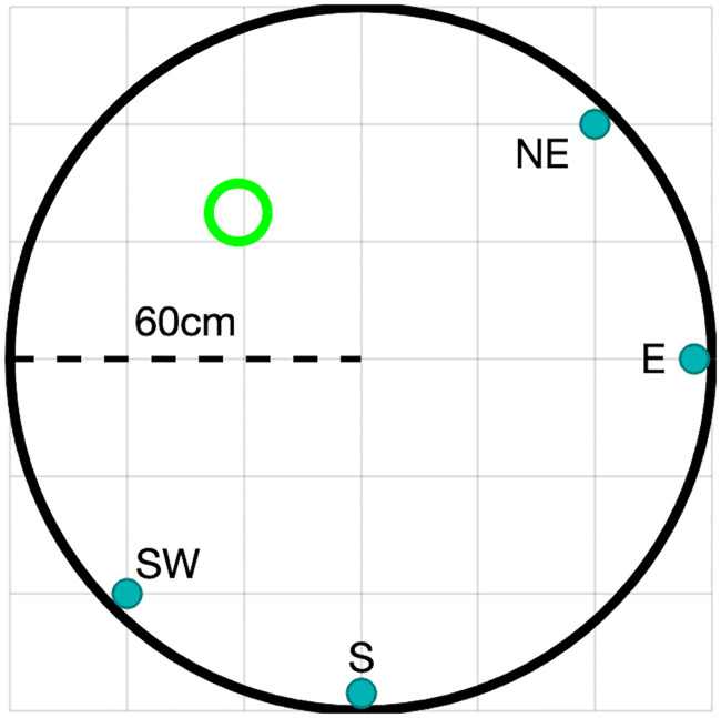
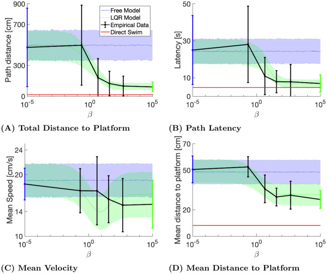
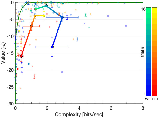
We introduce a novel methodology for describing animal behavior as a tradeoff between value and complexity, using the Morris Water Maze navigation task as a concrete example. We develop a dynamical system model of the Water Maze navigation task, solve its optimal control under varying complexity constraints, and analyze the learning process in terms of the value and complexity of swimming trajectories. The value of a trajectory is related to its energetic cost and is correlated with swimming time. Complexity is a novel learning metric which measures how unlikely is a trajectory to be generated by a naive animal. Our model is analytically tractable, provides good fit to observed behavior and reveals that the learning process is characterized by early value optimization followed by complexity reduction. Furthermore, complexity sensitively characterizes behavioral differences between mouse strains.

Fig 1. The water maze experiment.

Schematic figure of the water maze experiment. The fixed platform is shown in green. Release locations are indicated near the tank’s perimeter.

Fig 2. Empirical and model generated trajectories.

Top: empirical trajectories generated by naive (day 1) mice (left) and simulated trajectories generated by the uncontrolled model (right). Bottom: empirical trajectories generated by trained (day 4) mice (left) and simulated trajectories generated by the optimal control model (right). Initial positions, indicated by filled squares, and velocities, were matched between empirical and simulated trajectories. Trajectories simulated by the uncontrolled model are confined to tank boundaries.

Fig 3. Model and empirical performance measures.

The first and last empirical data points represent the trials used for training the uncontrolled (blue) and optimal control (green) models. The four mid points (black) represent the four training days. The empirical points shown are for the E release location. Error bars indicate standard deviations. The shaded areas represent one standard deviation above and below the average computed from the simulated swimming paths. The red line in panels A, B and D correspond to the minimum achievable value for the corresponding parameter, computed using a straight swimming path from the release location to the platform, using the mean velocity over all trials from the corresponding release location.

Fig 4. Model predictions along a trajectory as a function of β.

Actual and model predicted vectors for different β values shown at several points along an empirical path from the first day starting at the S release location. The black arrows represent the actual velocity vectors at the same point. Model predicted vectors corresponding to large β values (red and yellow arrows), are better oriented towards the platform than the those corresponding to smaller β values (blue and green). The non-monotonic speed profile (arrow length) as a function of beta can be seen in the top inset (red border). The standard deviation of the velocity noise is shown as a grey circle around the tip of the predicted velocity vector in the bottom inset (blue border). The velocity vectors corresponding to the estimated value of β that best fits the data (β = 0.273) are indicated by dashed black arrows in the insets.

Fig 5. Value-complexity curve.

Each point represents an empirical trajectory from a single release location (N). The axes show the value (ordinate) and complexity (abscissa) of each trajectory with the theoretically optimal curve plotted in green. Complexity tended to be lower for the mutant (heterozygous) animals compared to the wildtypes (warm and cool color scales respectively), and more so for females (circles) than for males (squares). While mean value tended to increased monotonically with training for both mutant and wildtype females (warm and cool gradient lines respectively), the mean complexity of wildtype females exhibited a non-monotonic profile, increasing on days 1-3 and decreasing on day 4. Trials from all six mouse batches are superimposed, with color hue indicating serial position within each batch. Large circles represent the daily mean value and complexity levels of wildtype (cool colors) and mutant (warm colors) female mice. Error bars are displayed for every 5th trial to reduce visual clutter.

Fig 6. Trajectory statistics.

Median path latency, value and complexity (ordinate) vs. trial day (abscissa) for female (top) and male (bottom) mice. Bottom and top bar edges indicate the 25th and 75th percentiles respectively. To reduce heteroscedasticity, ordinate data was transformed using a Box-Cox transform with power coefficients of: −0.29, 0.20, −0.19 (for latency, value and complexity data respectively).

Fig 7. Flotation behavior.

Trajectories of female (top) and male (bottom) wildtype (left) and heterozygous (right) mice released at the NE location. Blue circles indicate trajectory segments in which the speed of the mice was slower than 10% of the mean velocity along the trajectory.

References

1. Sutton RS, Barto AG, et al. Reinforcement learning: An introduction. MIT press; 1998.
1. Morris RGM. Spatial localization does not require the presence of local cues. Learning and Motivation. 1981;12(2):239–260. 10.1016/0023-9690(81)90020-5 - DOI
1. Gallagher M, Burwell R, Burchinal M. Severity of Spatial Learning Impairment in Aging: Development of a Learning Index for Performance in the Morris Water Maze Measures Traditionally Used for Behavioral Analysis in the Water Maze. Behavioral Neurosctence. 1993;107(4):8–626. Available from: https://www.brown.edu/research/labs/burwell/sites/brown.edu.research.lab.... - PubMed
1. Bryson AE. Applied optimal control: optimization, estimation and control. CRC Press; 1975.
1. Cover TM, Thomas JA. Elements of information theory. John Wiley & Sons; 2012.
Publication types
LinkOut - more resources