Reference ranges ("normal values") for cardiovascular magnetic resonance (CMR) in adults and children: 2020 update

Abstract

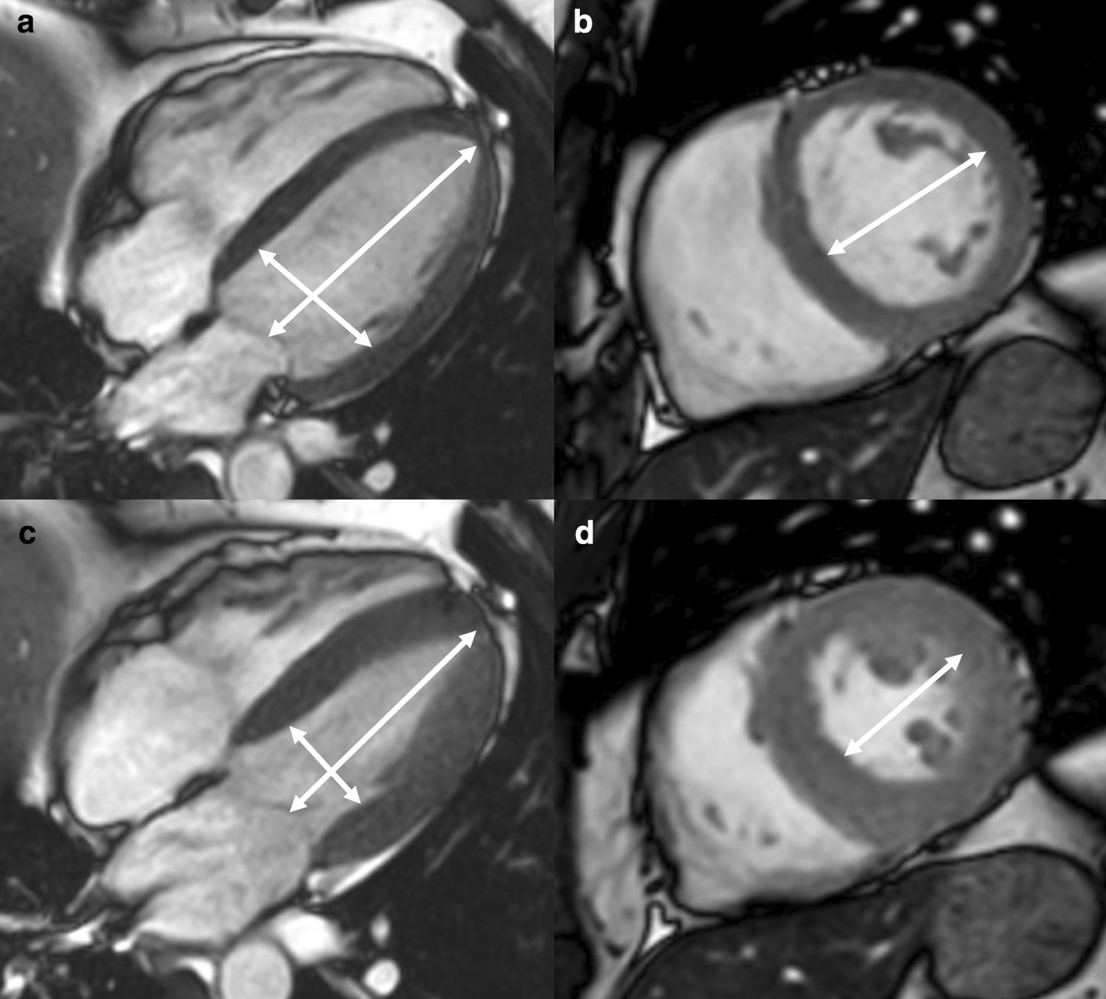
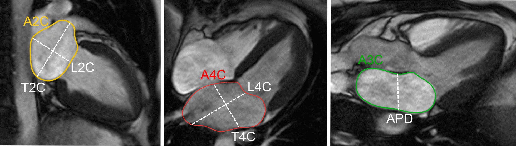
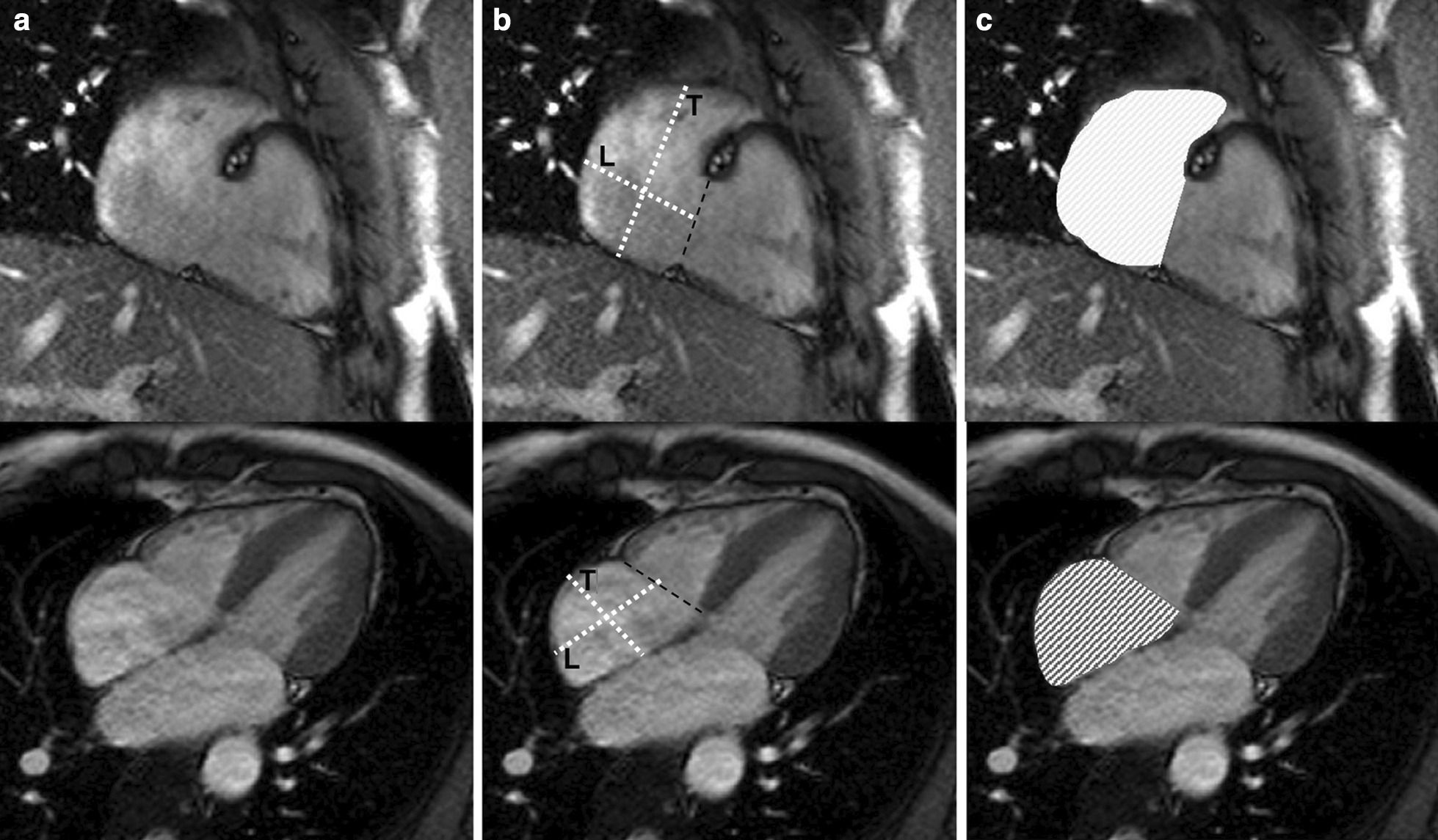
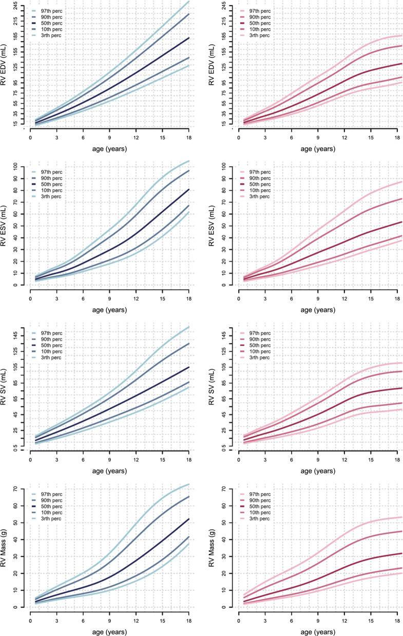
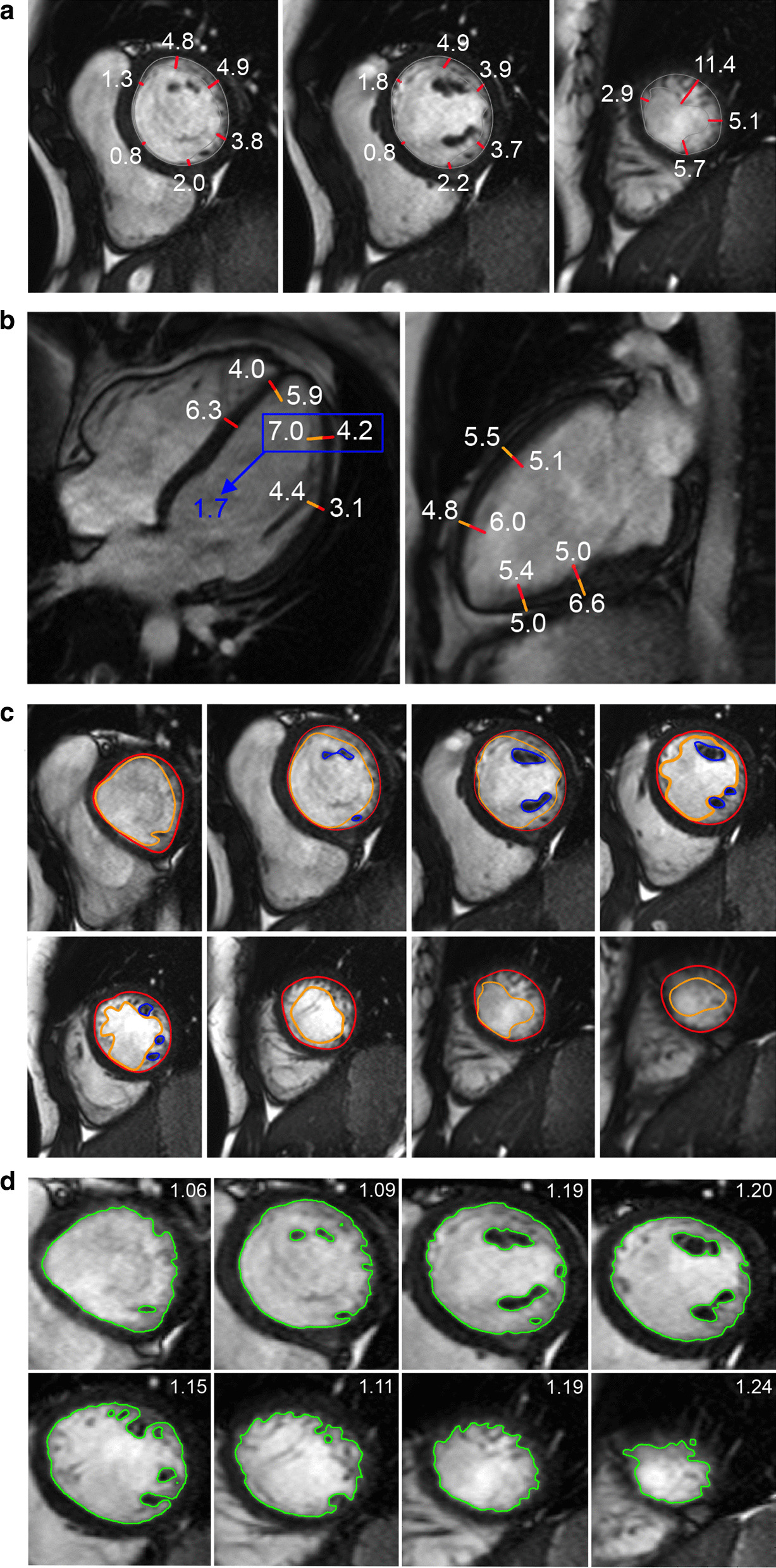
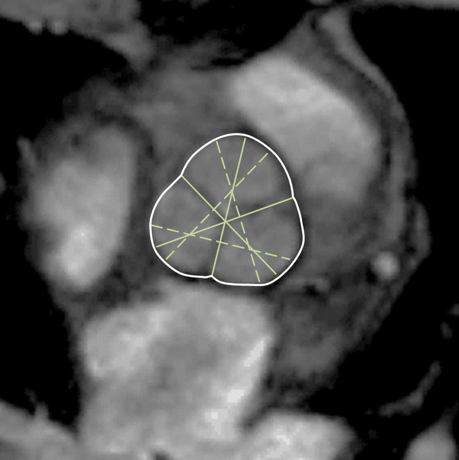
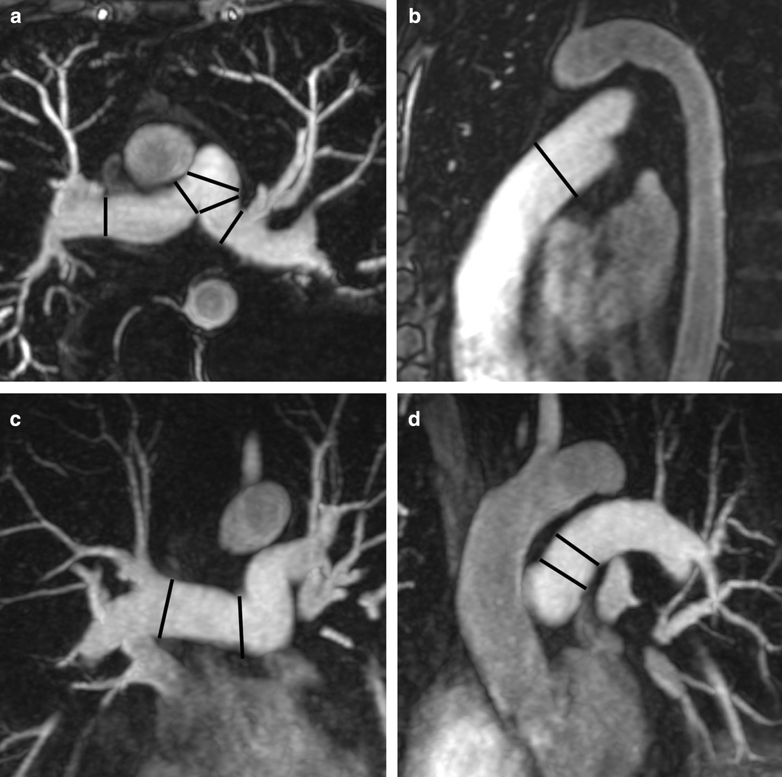
Cardiovascular magnetic resonance (CMR) enables assessment and quantification of morphological and functional parameters of the heart, including chamber size and function, diameters of the aorta and pulmonary arteries, flow and myocardial relaxation times. Knowledge of reference ranges ("normal values") for quantitative CMR is crucial to interpretation of results and to distinguish normal from disease. Compared to the previous version of this review published in 2015, we present updated and expanded reference values for morphological and functional CMR parameters of the cardiovascular system based on the peer-reviewed literature and current CMR techniques. Further, databases and references for deep learning methods are included.

Keywords: Cardiac magnetic resonance; Normal values; Reference range.

Fig. 1

Contouring of the left ventricle (LV) and right ventricle (RV). Note that LV papillary muscle mass has been isolated and added to LV mass. RV papillary muscles and trabeculations were included in the RV volume

Fig. 2

Measurements of LV diameters obtained on cine bSSFP images during diastole (a, b) and systole (c, d) on the 4 chamber view (a, c) and short axis view (b, d). The longitudinal diameter of the LV was measured on the 4 chamber view as the distance between the mitral valve plane and the LV apex (a, c). On the 4 chamber view the transverse diameter was defined as the distance between the septum and the lateral wall at the basal level [18]. On the short axis view the transverse diameter was obtained at the level of the basal papillary muscles (b, d) [15]

Fig. 3

Measurement of left atrial area (A2Ch, A4Ch, A3C), longitudinal (L2Ch, L4Ch), transverse (T2Ch, T4Ch) and anteroposterior (APD) diameters on the 2-, 4- and 3-chamber views according to reference [31]

Fig. 4

Measurement of right atrial (RA) parameters according to [37]. Areas and diameters were measured in atrial diastole (maximal size of the left atrium) on the 2-chamber (top row) and 4-chamber (bottom row) views. In B), longitudinal diameter (L) is obtained from the posterior wall of the RA to the center of the tricuspid plane, and transverse diameter (T) is obtained perpendicular to the longitudinal diameter, at the mid level of the RA. C shows measurements of the area for both views including the RA appendage

Fig. 5

Reference curves for LV dimensions and function in children, reprinted with permission from reference [45]. Curves for boys are displayed in blue on the left, curves for girls are shown in pink on the right. Reference lines show the 3rd, 10th, 90th and 97th percentile. LV left ventricle, ED end diastolic, ES end systolic, SV stroke volume

Fig. 6

Reference curves for RV dimensions and function in children, reprinted with permission from reference [45]. Curves for boys are displayed in blue on the left, curves for girls are shown in pink on the right. Reference lines show the 3rd, 10th, 90th and 97th percentile. LV left ventricle, ED end diastolic, ES end systolic, SV stroke volume

Fig. 7

Example of measurement approaches for LV trabeculation. a End-diastolic thickness (in mm) of trabeculation according to the methodology in [56]: 3 slices representing base, mid and apex were selected from within the entire LV stack; trabeculated myocardial thickness was measured per slice; segment 17 excluded from analysis; authors do not clarify whether papillary muscles had been included or excluded from the trabecular measurement—in this reproduction we have excluded papillary muscles. b Maximal non-compacted (NC, red lines)/compacted (c, orange lines) wall thickness ratio according to the methodology in [61]: papillary muscles that were clearly observed as compact tubular structures were not included in the measurements; measurements in mm are shown in white and the maximal NC/C parameter highlighted in blue. c Trabeculation mass according to the methodology in [12]: the endocardial contour (red) was manually drawn; the trabecular contour (orange) was automatically segmented and papillary muscles (blue) that were included in the compact myocardial mass, were semi-automatically segmented; all slices of the LV short axis stack were analyzed. d Fractal dimension according to the methodology in [60]: using a semi-automatic level-set segmentation with bias field correction; all slices of the LV short axis stack are analyzed except for the apical slice; fractal dimensions per slice reported in the top right corner

Fig. 8

Images of a 4D flow sequence illustrating sites of measurement of peak systolic velocity. According to reference [77] measurements were obtained where the transvalvular velocity reaches its maximum during peak systole (vena contracta region) (a). In reference [76] peak systolic velocity was obtained in the ascending aorta 6 cm proximal from the most cranial point of the aortic arch centerline (b)

Fig. 9

Sites of measurement of the thoracic aorta. AS aortic sinus, STJ sinotubular junction, AA ascending aorta, BCA proximal to the origin of the brachiocephalic artery, T1 between the origin of the brachiocephalic artery and the left common carotid artery, T2 between the origin of the left common carotid artery and the left subclavian artery, IR isthmic region, DA descending aorta, D thoracoabdominal aorta at the level of the diaphragm

Fig. 10

Measurements of luminal diameters of the aortic annulus (a), the aortic sinus (b) and the sinotubular junction (c) obtained on a steady-state free precession left ventricular outflow tract view at diastole according to reference [86]

Fig. 11

Cusp-commissure (continuous lines) and cusp-cusp (dashed-lines) measurements at the level of the aortic sinus according to reference [85]

Fig. 12

Measurement of pulse wave velocity according to reference [92]. Δx: length of the centerline between the sites of flow measurement in the ascending and descending aorta; Δt: time delay between the flow curves obtained in the descending aorta relative to the flow curve obtained in the ascending aorta calculated between the midpoint of the systolic up slope tails on the flow versus time curves of the ascending aorta (ta1) and the descending aorta (ta2)

Fig. 13

Measurement of the dimensions of the pulmonary arteries on bSSFP images according to [99]. Oblique sagittal image of the main pulmonary artery (a). The pale band in a shows the acquisition plane of the cross sectional image of the main pulmonary artery in b. Right and left pulmonary arteries on the scout image (c) with band indicating the location of cine acquisitions transecting the right (d) and left (e) pulmonary artery

Fig. 14

Measurement of the diameters of the pulmonary arteries according to reference [100]. Diameters were measured perpendicular to the vessel on maximum intensity projection images. The diameters of the main pulmonary artery were obtained on an axial (a) and sagittal oblique (b) view and the diameters of the proximal and distal right and left pulmonary artery were obtained on axial (a) and right and left anterior oblique (paracoronal) views (c, d), respectively

Fig. 15

T1 maps with measurements. T1 map pre- (a) and post-contrast (b) with left ventricular endocardial and epicardial contours according to reference [119]

Fig. 16

Measurements of myocardial T2* are obtained in the septum

Fig. 17

Illustration of strain computation using the Harmonic Phase (HARP) tool on tagged CMR images (a–d) and from feature tracking on cine CMR images (e–h). In HARP, first a semi-automated frequency analysis of the tagged CMR image (a) is performed to identify the harmonic peaks in each of the tag directions (b), filters are then applied to isolate the peaks and obtain the corresponding phase maps from which Eulerian strain maps (c) can be computed. Subplot (d) shows the strain curve at the mid-ventricular level for an asymptomatic volunteer obtained based on tracking of the user-defined mesh (a). In feature tracking of cine CMR images, endo- and epicardial contours are drawn at end-diastole (e) or end-systole (g). A characteristic pixel pattern in the order of a few millimeters squared is identified as a template. The software then tries to discern a similar pattern in the subsequent frame from which displacement of the pixels is computed (f). This is repeated through the entire cycle to obtain displacement from which strain is computed. Subplot (h) shows the strain curve at the mid-ventricular level computed from feature tracking. The tagged and cine CMR images and the strain curves were from the same participant

Fig. 18

a The quantification of myocardial perfusion proceeds from the segmentation of images acquired during the first pass of contrast through the heart to delineate myocardial segments and a region in the center of the LV blood pool for the arterial input. This example shows one short-axis image for a mid-slice LV level. b For each myocardial segment one obtains a signal-intensity versus time curve. A useful semi-quantitative parameter for the assessment of the perfusion in a myocardial segment is the upslope, which is estimated from a fit to approximately 3–5 points during the initial myocardial contrast enhancement. c An analogous upslope parameter can be extracted from the first pass peak of the arterial input function. A perfusion index can be calculated from the ratio of the two upslopes as shown in the formula below (a), and accounts for some changes in the arterial input between rest and stress. d Absolute estimates of myocardial blood flow in ml/min/g can be obtained from the myocardial contrast enhancement curves and the arterial input function by fitting to a kinetic model for contrast enhancement, or, as done for this example, to estimate the myocardial impulse response by constrained deconvolution. Constraints are that the impulse response should be a monotonically decaying function of time, and requiring a relatively smooth, “regularized” impulse response. Myocardial blood flow (MBF) is estimated from the peak amplitude of the impulse response. e The ratio of myocardial blood flows during stress, divided by MBF at rest provides the most accurate estimate of the coronary flow reserve. In comparison, other ratios of perfusion indices (e.g. upslope index) for stress and rest systematically underestimate the flow reserve but may still prove useful for the detection of disease, assuming that one has established the normal range of the index.

References

1. Kawel-Boehm N, Maceira A, Valsangiacomo-Buechel ER, Vogel-Claussen J, Turkbey EB, Williams R, Plein S, Tee M, Eng J, Bluemke DA. Normal values for cardiovascular magnetic resonance in adults and children. J Cardiovasc Magn Reson. 2015;17:29. doi: 10.1186/s12968-015-0111-7. - DOI - PMC - PubMed
1. Bai W, Sinclair M, Tarroni G, Oktay O, Rajchl M, Vaillant G, Lee AM, Aung N, Lukaschuk E, Sanghvi MM, et al. Automated cardiovascular magnetic resonance image analysis with fully convolutional networks. J Cardiovasc Magn Reson. 2018;20:65. doi: 10.1186/s12968-018-0471-x. - DOI - PMC - PubMed
1. Tao Q, Yan W, Wang Y, Paiman EHM, Shamonin DP, Garg P, Plein S, Huang L, Xia L, Sramko M, et al. Deep Learning-based Method for Fully Automatic Quantification of Left Ventricle Function from Cine MR Images: A Multivendor Multicenter Study. Radiology. 2019;290:81–88. doi: 10.1148/radiol.2018180513. - DOI - PubMed
1. Horowitz GL. Estimating reference intervals. Am J Clin Pathol. 2010;133:175–177. doi: 10.1309/AJCPQ4N7BRZQVHAL. - DOI - PubMed
1. SCMR: Consensus/Position statements, [https://scmr.org/general/custom.asp?page=guidelines], Accessed 15 Dec 2019
Publication types