Exact neural mass model for synaptic-based working memory

Abstract

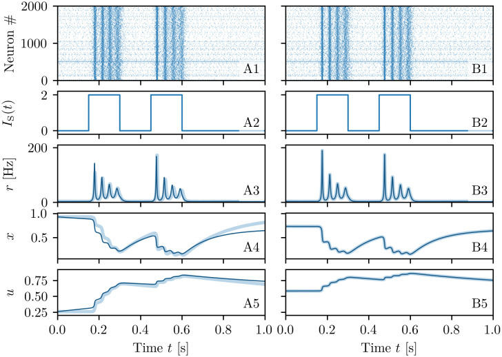
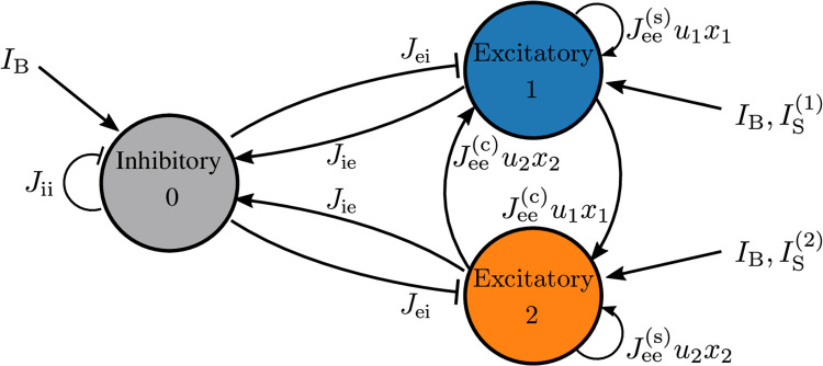
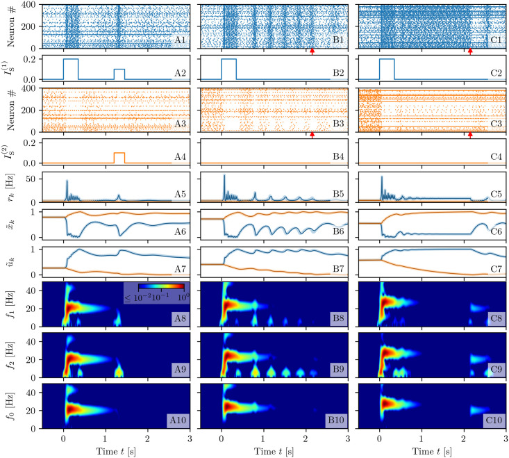
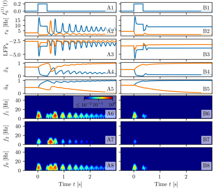
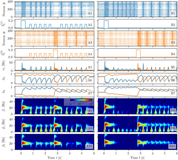
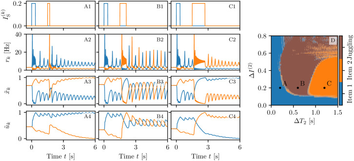
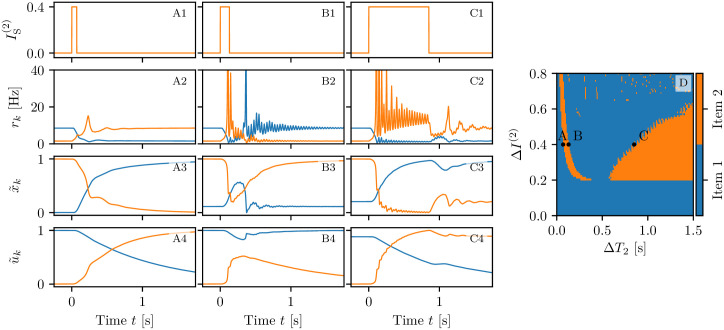
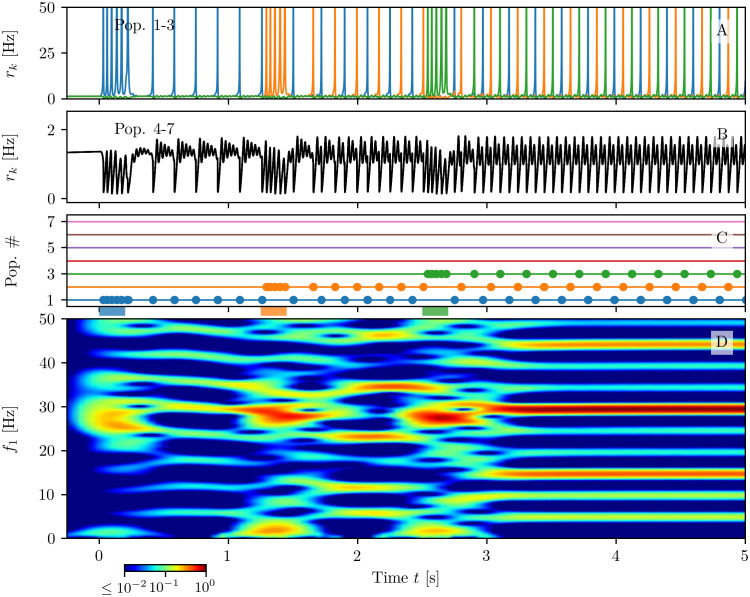
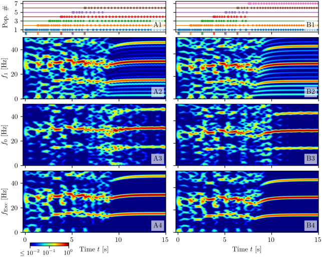
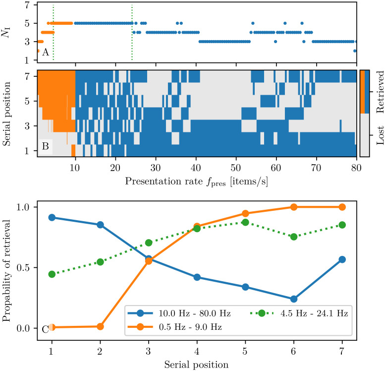
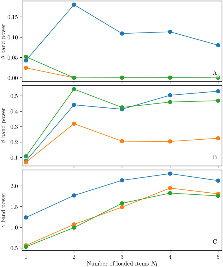
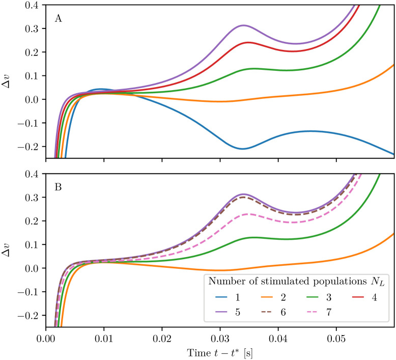
A synaptic theory of Working Memory (WM) has been developed in the last decade as a possible alternative to the persistent spiking paradigm. In this context, we have developed a neural mass model able to reproduce exactly the dynamics of heterogeneous spiking neural networks encompassing realistic cellular mechanisms for short-term synaptic plasticity. This population model reproduces the macroscopic dynamics of the network in terms of the firing rate and the mean membrane potential. The latter quantity allows us to gain insight of the Local Field Potential and electroencephalographic signals measured during WM tasks to characterize the brain activity. More specifically synaptic facilitation and depression integrate each other to efficiently mimic WM operations via either synaptic reactivation or persistent activity. Memory access and loading are related to stimulus-locked transient oscillations followed by a steady-state activity in the β-γ band, thus resembling what is observed in the cortex during vibrotactile stimuli in humans and object recognition in monkeys. Memory juggling and competition emerge already by loading only two items. However more items can be stored in WM by considering neural architectures composed of multiple excitatory populations and a common inhibitory pool. Memory capacity depends strongly on the presentation rate of the items and it maximizes for an optimal frequency range. In particular we provide an analytic expression for the maximal memory capacity. Furthermore, the mean membrane potential turns out to be a suitable proxy to measure the memory load, analogously to event driven potentials in experiments on humans. Finally we show that the γ power increases with the number of loaded items, as reported in many experiments, while θ and β power reveal non monotonic behaviours. In particular, β and γ rhythms are crucially sustained by the inhibitory activity, while the θ rhythm is controlled by excitatory synapses.

Fig 1. Comparison among neural mass and network models.

The results of the neural mass model (solid line) are compared with the network simulations (shaded lines) for a single excitatory population with μ-STP (column A) and with m-STP (column B). The corresponding raster plots for a subset of 2000 neurons are reported in (A1-B1), the profiles of the stimulation current I_S(t) in (A2-B2), the instantaneous population firing rates r(t) in (A3-B3), the available synaptic resources x(t) in (A4-B4), and the utilization factors u(t) in (A5-B5). The variables of the neural mass model are initialized to values coinciding with those of the corresponding network simulations. Since the numerical experiments for the single excitatory population with μ-STP (column A) and with m-STP (column B) are independent, the initial values of the synaptic variables do not coincide, even though a similar dynamical evolution is observable in both cases. Simulation parameters are ${\tau }_m^e=15$ ms, H = 0, Δ = 0.25, J = 15, I_B = −1 and network size N = 200, 000.

Fig 2. Two-item architecture.

The reported network is composed of two identical and mutually coupled excitatory populations and an inhibitory one: this architecture can at most store two WM items, one for each excitatory population.

Fig 3. Memory loading, maintenance and rehearsal.

The results of three experiments are reported here for different background currents: selective reactivation of the target population (I_B = 1.2, A); WM maintenance via spontaneous reactivation of the target population (I_B = 1.532, B) and via a persistent asynchronous activity (I_B = 2, C). Raster plots of the network activity for the first (blue, A1-C1) and second (orange, A3-C3) excitatory population; here the activity of only 400 neurons over 200,000 ones is shown for each population. Profiles of the stimulation current $I_S^{(k)}(t)$ for the first (A2-C2) (second (A4-C4)) excitatory population. Population firing rates r_k(t) (A5-C5), normalized available resources ${\tilde{x}}_k(t)$ (A6-C6) and normalized utilization factors ${\tilde{u}}_k(t)$ (A7-C7) of the excitatory populations calculated from the simulations of the neural mass model (solid line) and of the network (shading). Spectrograms of the mean membrane potentials v₁(t) (A8-C8), v₂(t) (A9-C9), and v₀(t) (A10-C10) obtained from the neural mass model; for clarity the frequencies in these three cases have been denoted as f₁, f₂ and f₀, respectively. Red arrows in columns (B) and (C) indicate the time t = 2.15 s at which the background current is set to the value I_B = 1.2 employed in column (A). The network simulations have been obtained by considering three populations of N = 200, 000 neurons each (for a total of 600,000 neurons) arranged with the architecture displayed in Fig 2. Other parameters: ${\tau }_m^e=15$ ms H⁽ⁱ⁾ = H^(e) = 0, Δ⁽ⁱ⁾ = Δ^(e) = 0.1, $J_{ee}^{(c)}=5\sqrt{a}$, $J_{ee}^{(s)}=35\sqrt{a}$, $J_{ie}=13\sqrt{a}$, $J_{ei}=-16\sqrt{a}$, $J_{ii}=-14\sqrt{a}$ with a = 0.4.

Fig 4. WM operations for a heuristic firing rate model.

The results of two experiments are reported here for different background currents: WM maintenance via spontaneous reactivation of the target population (I_B = 1.520, A) and via a persistent asynchronous activity (I_B = 2.05, B). Profiles of the stimulation current $I_S^{(k)}(t)$ for the excitatory populations (A1-B1). Population firing rates r_k(t) (A2-B2), local field potentials LFP_k defined in Eq (28) (A3-B3), normalized available resources ${\tilde{x}}_k(t)$ (A4-C4) and normalized utilization factors ${\tilde{u}}_k(t)$ (A5-C6) of the excitatory populations calculated from simulations of the firing rate model (19), (21). Spectrograms of the local field potentials: LFP₁(t) (A6-B6), LFP₂(t) (A7-B7), and LFP₀(t) (A8-B8). All the other parameter values as in Fig 3.

Fig 5. Juggling between two memory items.

The memory juggling is obtained in two experiments with different background currents: in presence of a periodic unspecific stimulation (I_B = 1.2, A) and in the case of spontaneous WM reactivation (I_B = 1.532, B). Raster plots of the network activity for the first (blue, A1-B1) and second (orange, A3-B3) excitatory population. Profiles of the stimulation current $I_S^{(k)}(t)$ for the first (A2-B2) (second (A4-B4))) excitatory population. Population firing rates r_k(t) (A5-B5), normalized available resources ${\tilde{x}}_k(t)$ (A6-B6) and normalized utilization factors ${\tilde{u}}_k(t)$ (A7-B7) of the excitatory populations calculated from the simulations of the neural mass model (solid line) and of the network (shading). Spectrograms of the mean membrane potentials v₁(t) (A8-B8), v₂(t) (A9-B9), and v₀(t) (A10-B10) obtained from the neural mass model. All the other parameter values as in Fig 3.

Fig 6. Competition between two memory items.

The loading of two memory items is performed in three different ways via two step currents of equal amplitudes ΔI⁽¹⁾ = ΔI⁽²⁾ = 0.2, the first one delivered at t = 0 and the second one at t = 1.5 s. The first step has always a duration of ΔT₁ = 0.35 s; the second one ΔT₂ = 0.2 s (column A), ΔT₂ = 0.6 s (column B) and ΔT₂ = 1.2 s (column C). Stimulation currents $I_S^{(k)}(t)$ (A1-C1), instantaneous population firing rates r_k(t) (A2-C2), normalized available resources ${\tilde{x}}_k(t)$ (A3-C3) and normalized utilization factors ${\tilde{u}}_k(t)$ (A4-C4) for the first (blue) and second (orange) excitatory population. Final memory states as a function of the amplitude ΔI⁽²⁾ and width ΔT₂ of the stimulus to population two (D). In (D) the three letters A, B, C refer to the states examined in the corresponding columns. The data reported in panel (D) has been obtained by delivering the second stimulation at different phases φ with respect to the period of the CO of the first population: 20 equidistant phases in the interval ϕ ∈ [0, 2π) have been considered. For each of the three possible outcomes an image has been created with a level of transparency corresponding to the fraction of times it has been measured. The three images have been merged resulting in panel (D). All the other parameter values as in Fig 3, apart for I_B = 1.532.

Fig 7. Memory item switching with persistent activity.

The three columns (A-C) refer to three values of ΔT₂ for which we have a memory switching from one item to the other for a background current I_B = 2 supporting persistent state activity. (A) ΔT₂ = 70 ms; (B) ΔT₂ = 130 ms and (C) ΔT₂ = 850 ms. Profiles of the stimulation current $I_S^{(2)}(t)$ for the second excitatory population (A1-C1). Population firing rates r_l(t) (A2-C2), normalized available resources ${\tilde{x}}_l(t)$ (A3-C3) and normalized utilization factors ${\tilde{u}}_l(t)$ (A4-C4) of the excitatory populations calculated from the simulations of the neural mass model. Final memory states as a function of the amplitude ΔI⁽²⁾ and width ΔT₂ of the stimulus to population two (D). In (D) the three letters A, B, C refer to the states examined in the corresponding columns. Other parameters as in Fig 3, apart for I_B = 2.

Fig 8. Multi-item memory loading.

Firing rates r_k(t) of excitatory populations: blue, orange and green curves corresponds to k = 1, 2, 3 (A), while the black curve refers to k = 4, …, 7 (B). PBs of excitatory populations are shown in (C): horizontal lines in absence of dots indicate low activity regimes; coloured dots mark the PBs’ occurrences. The coloured bars on the time axis denote the presence of a stimulation pulse targeting the corresponding population. Only populations k = 1, …, 3 are stimulated in the present example. The spectrogram of the average membrane potential of population one v₁(t) is reported in panel (D). Parameters: N_pop = 7, ${\tau }_m^e=15$ ms, ${\tau }_m^i=10$ ms, $J_{ee}^{(s)}=154$, $J_{ee}^{(c)}=\frac{4}{7}\cdot 18.5$, J_ei = −26, $J_{ie}=\frac{4}{7}\cdot 97$, J_ii = −60, I_B = 0, H^(e) = 0.05, H⁽ⁱ⁾ = −2, Δ^(e) = Δ⁽ⁱ⁾ = 0.1.

Fig 9. Maximal capacity.

Response of the system when N_L = 6 (column (A)) or N_L = 7 (column (B)) excitatory populations are successively stimulated at a presentation rate of 0.8 Hz. Population bursts of excitatory populations (A1-B1): horizontal lines in absence of dots indicate quiescence phases at low firing rates r_k for populations k = 1, …7. Dots mark PBs of the corresponding population. The coloured bars on the time axis mark the starting and ending time of stimulating pulses, targeting each population. Spectrograms of the mean membrane potential v₁(t) (A2-B2), v₀(t) (A3-B3) and of the mean membrane potentials averaged over all the excitatory populations (A4-B4); for clarity the corresponding frequencies have been denoted as f₁, f₀ and f_Exc. Parameter values as in Fig 8.

Fig 10. Dependence of the memory capacity on the presentation rate.

(A) Total number of retrieved items N_I vs. presentation frequency f_pres for slow ([0.5: 9.0] Hz, orange) and fast presentation rates ([10: 80] Hz, blue). The two green dotted vertical lines denote an optimal rate interval where N_I is maximal. (B) Map showing the retrieved items at a given serial position for presentation rates f_pres in the interval [0.5: 80] Hz. (C) Probability of retrieval vs. serial position for slow (orange) and fast (blue) presentation rates. In order to estimate these probabilities 150 equidistant rates are considered in the interval [0.5: 9] Hz and 150 in [10, 80] Hz. The green dotted line refers to the probability estimated within the rate interval enclosed between two green dotted vertical lines in (A). An item is considered as retrieved if the corresponding population is still delivering PBs 20 s after the last stimulation. All other parameter values are as in Fig 8.

Fig 11. Dependence of the power on the number of loaded items.

Power in the θ-band (3-11 Hz) (A), in the β-band (11-25 Hz) (B) and in the γ-band (25-100 Hz) (C) as a function of the number N_L = N_I ≤ 5 of loaded items. The integral of the power spectra in the specified frequency bands are displayed for the mean membrane potential v₁(t) of the excitatory population one (blue symbols), the mean membrane potential v₀(t) of the inhibitory population (orange symbols) and the mean membrane potentials averaged over all the excitatory populations (green symbols). The power spectra have been evaluated over a 10 s time window, after the loading of N_I items, when these items were juggling in WM. Parameter values as in Fig 8.

Fig 12. Dependence of the membrane potential difference on the number of loaded items.

Difference Δv of membrane potentials versus time when stimulating different numbers N_L of populations. The presented time-series are aligned to t*, which marks the deliverance of a PB from population one. The populations are stimulated sequentially with parameter values as in Fig 8.

Fig 13. Bifurcation diagram for two excitatory populations.

Bifurcation diagram displaying the instantaneous firing rates r_k (A) and mean membrane potentials v_k (B) for the excitatory populations as a function of the background current I_B. Solid (dashed) black lines refer to stable (unstable) asynchronous states, while green solid lines denote the maxima and the minima of stable collective oscillations. Symbol refer to bifurcation points: branch points (blue squares), Hopf bifurcations (orange circles) and saddle-node bifurcations (red circles). The inset in (A) displays an enlargement of the bifurcation diagram. The lower (upper) branch of equilibria in (A) corresponds to the lower (upper) branch in (B). All the remaining parameters are as in Fig 3. Continuation performed with the software AUTO-07P [82].

References

1. Just MA, Carpenter PA. A capacity theory of comprehension: individual differences in working memory. Psychological review. 1992;99(1):122 10.1037/0033-295X.99.1.122 - DOI - PubMed
1. Goldman-Rakic PS. Cellular basis of working memory. Neuron. 1995;14(3):477–485. 10.1016/0896-6273(95)90304-6. - DOI - PubMed
1. Engle RW, Tuholski SW, Laughlin JE, Conway AR. Working memory, short-term memory, and general fluid intelligence: a latent-variable approach. Journal of experimental psychology: General. 1999;128(3):309 10.1037/0096-3445.128.3.309 - DOI - PubMed
1. Fuster JM. Memory in the cerebral cortex: An empirical approach to neural networks in the human and nonhuman primate. MIT press; 1999.
1. Vogel EK, Machizawa MG. Neural activity predicts individual differences in visual working memory capacity. Nature. 2004;428(6984):748–751. 10.1038/nature02447 - DOI - PubMed
Publication types