Metapangenomics of the oral microbiome provides insights into habitat adaptation and cultivar diversity

Abstract

Background: The increasing availability of microbial genomes and environmental shotgun metagenomes provides unprecedented access to the genomic differences within related bacteria. The human oral microbiome with its diverse habitats and abundant, relatively well-characterized microbial inhabitants presents an opportunity to investigate bacterial population structures at an ecosystem scale.

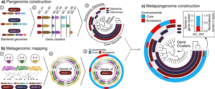
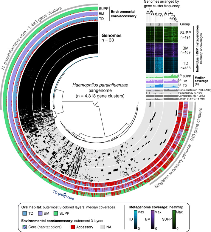
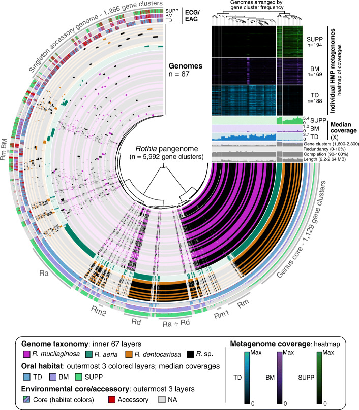
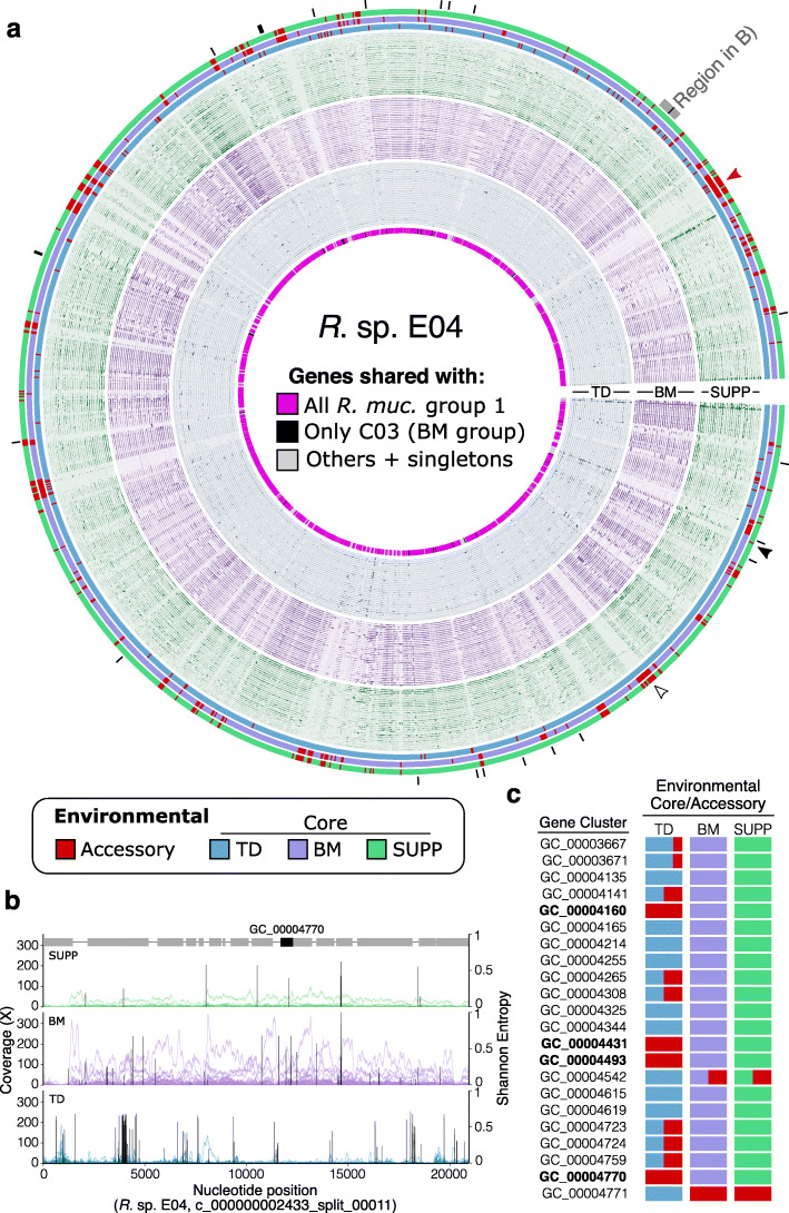
Results: Here, we employ a metapangenomic approach that combines public genomes with Human Microbiome Project (HMP) metagenomes to study the diversity of microbial residents of three oral habitats: tongue dorsum, buccal mucosa, and supragingival plaque. For two exemplar taxa, Haemophilus parainfluenzae and the genus Rothia, metapangenomes reveal distinct genomic groups based on shared genome content. H. parainfluenzae genomes separate into three distinct subgroups with differential abundance between oral habitats. Functional enrichment analyses identify an operon encoding oxaloacetate decarboxylase as diagnostic for the tongue-abundant subgroup. For the genus Rothia, grouping by shared genome content recapitulates species-level taxonomy and habitat preferences. However, while most R. mucilaginosa are restricted to the tongue as expected, two genomes represent a cryptic population of R. mucilaginosa in many buccal mucosa samples. For both H. parainfluenzae and the genus Rothia, we identify not only limitations in the ability of cultivated organisms to represent populations in their native environment, but also specifically which cultivar gene sequences are absent or ubiquitous.

Conclusions: Our findings provide insights into population structure and biogeography in the mouth and form specific hypotheses about habitat adaptation. These results illustrate the power of combining metagenomes and pangenomes to investigate the ecology and evolution of bacteria across analytical scales.

Keywords: Biogeography; Haemophilus parainfluenzae; Metagenomes; Oral microbiome; Pangenomes; Population structure; Rothia.

Fig. 1

Metapangenomic workflow. a Pangenome construction. (1) All putative protein-coding gene sequences (colored block arrows) are extracted from each bacterial genome (colored bacilli above genes) to be included in the pangenome and (2) clustered into homologous gene clusters via blastp results grouped by the Markov Clustering Algorithm (sequence variants cartoonized as shades of the same color). (3) These gene clusters become the central dendrogram of the pangenome. Note that the gene clusters are organized by occurrence in genomes, not based on the order found in a particular genome. The detection of each gene cluster in a genome is visualized by filling in to indicate the presence or absence of each gene cluster across the genomes. The genomes are ordered by a dendrogram (top right) based on each genome’s gene cluster content. b Metagenomic mapping. (1) The exact genomes as above in a are used as a reference onto which reads from metagenomes are mapped. Gene-level coverage for each gene is then calculated. (2) These coverages are plotted for all genes from a given genome to show that genome’s gene-level representation in those samples. (3) Environmental representation is evaluated for each gene to decide whether that gene is environmentally core (gene’s median coverage > 0.25 of the genome’s median coverage across metagenomes from that environment) or environmentally accessory (gene’s median coverage < 0.25 of the genome’s median coverage). c Metapangenome construction. The environmental representation from b is then summarized for all genes and then overlaid onto the pangenome created in a—the inner layers show the genomic representation of the pangenome, and the outer layer shows the environmental representation of the pangenome. This outer layer summarizes the fraction of genes in each gene cluster that were environmentally core or accessory in those metagenomes (callout)

Fig. 2

Metapangenomic analysis of Haemophilus parainfluenza reveals hidden diversity and habitat-specific subgroups. The inner radial dendrogram shows the 4318 gene clusters in the pangenome, clustered by presence/absence across genomes. The 33 genomes of H. parainfluenzae strains are plotted on the innermost 33 layers (black 270° arcs), spaced to reflect discernable groups based on genomic composition. Gene clusters within a given genome are filled in with black; gene clusters not present remain unfilled. Genomes are ordered by gene cluster frequency (top right dendrogram), with radial spacing added between major groups to improve visibility. The outermost three layers show the proportion of genes within each gene cluster determined to be environmental accessory (red) or core in HMP metagenomes from TD (blue), BM (violet), and SUPP (green), from inside to outside, respectively. If a genome was not well detected (< 0.5 of nucleotides covered by all metagenomes), all its genes were NA (gray) instead of environmentally core or accessory. Extending off the pangenome above 3 o’clock are bar charts of relevant information for each genome, with the y-axis limits in parentheses. Above the genome content summaries, each genome’s median coverage across all TD, BM, and SUPP metagenomes is shown in the colored bar graph. Per-sample coverage of each genome is shown in the heatmap above, where each row represents a different sample, and cell color intensity reflects the coverage. Coverage is normalized to the maximum value of that sample (black = 0, bright = maximum; colors as before for each site)

Fig. 3

Genomes in the Rothia genus metapangenome are organized by gene content into groups that reveal associations to specific habitats. Tips on the inner radial dendrogram, setting the angular axis, correspond to gene clusters organized by presence/absence across genomes. The angular distance thus holds the entirety of the Rothia pangenome, 5992 distinct gene clusters. The inner 67 layers (270° arcs) represent genomes, colored by NCBI’s taxonomic assignments, and are organized by their gene cluster frequencies (top right vertical dendrogram). Each genome’s gene cluster content is displayed by filling in cells (gene clusters) for genomes in which that gene cluster is present. Gaps in radial spacing of layers delineate major groups determined by inspection of the pangenome and dendrogram. Groups of gene clusters are annotated with text and a gray arc—“Genus core” are gene clusters core to the genus Rothia; “Rm,” R. mucilaginosa; “Rm1,” R. mucilaginosa subgroup 1; “Ra + Rd,” both R. aeria and R. dentocariosa; “Rd,” R. dentocariosa; “Rm2,” R. mucilaginosa subgroup 2; “Ra,” R. aeria; “Rm BM,” BM-abundant R. mucilaginosa. The outermost colored three layers show the proportion of genes within each gene cluster deemed environmental accessory (red) or core for HMP metagenomes from tongue dorsum (blue), buccal mucosa (violet), and supragingival plaque (green). If a genome was not well detected (< 0.5 of nucleotides covered by all metagenomes), all its genes were NA (gray) instead of environmentally core or accessory. Above the genome content summaries, each genome’s median coverage across all TD, BM, and SUPP metagenomes is shown in the colored bar graph. Per-sample coverage of each genome is shown in the heatmap above, where each row represents a different sample, and cell color intensity reflects the coverage. Coverage is normalized to the maximum value of that sample (black = 0, bright = maximum; colors as before for each site)

Fig. 4

Gene-scale metapangenomic analysis suggests candidate gene-level drivers of habitat adaptation. a Gene-level coverage of Rothia sp. E04. Units along the angular axis are R. sp. E04 genes, arranged in order found in R. sp. E04 with contigs joined arbitrarily. The innermost ring labels whether each gene was shared with all of R. mucilaginosa group 1 (pink), only between the BM-enriched strains R. spp. E04 and C03 (black; also shown with black lines outside figure), or otherwise (gray). The innermost 30 layers show coverage of each gene for 30 TD metagenomes with the highest coverage; middle 30, BM metagenomes; outer 30, SUPP metagenomes. Each layer’s y-axis shows coverage by an individual sample, with y-axes scaled independently for each layer. The three outermost layers show whether genes were determined as environmental accessory (red) or core in TD (blue), BM (violet), or SUPP (green). Arrowheads show examples of gene abundance patterns: uniformly low-to-absent coverage across metagenomes (empty black) vs stochastically abundant but typically environmentally accessory (filled black). b Nucleotide-level coverage for a 20-kb contiguous stretch of R. sp. E04’s genome that includes a candidate gene driver of the BM adaptation, GC_00004770. This stretch is shown by the labeled grey arc in a. Each trace shows a single sample’s coverage, colored according to its oral site. Black bars show the mean Shannon entropy for variant sites covered at least 10x. Gray boxes above the SUPP traces mark genes, with GC_00004770 highlighted in black. c Table of the 22 gene clusters unique to R. sp. E04 and R. sp. C03 (also marked with black ticks in panel a). The columns labeled “Environmental Core/Accessory” show the fraction of genes in each gene cluster that are core (colored according to that habitat’s color) or environmentally accessory (red). The corresponding Pfam function is listed for gene clusters for which a function could be predicted. The gene clusters environmentally core in BM and SUPP but not in TD are bolded

References

1. Human Microbiome Project Consortium A framework for human microbiome research. Nature. 2012;486(7402):215–221. doi: 10.1038/nature11209. - DOI - PMC - PubMed
1. Lloyd-Price J, Mahurkar A, Rahnavard G, Crabtree J, Orvis J, Hall AB, et al. Strains, functions and dynamics in the expanded Human Microbiome Project. Nature. 2017;550(7674):61. doi: 10.1038/nature23889. - DOI - PMC - PubMed
1. Tierney BT, Yang Z, Luber JM, Beaudin M, Wibowo MC, Baek C, et al. The landscape of genetic content in the gut and oral human microbiome. Cell Host Microbe. 2019;26(2):283–288. doi: 10.1016/j.chom.2019.07.008. - DOI - PMC - PubMed
1. Pasolli E, Asnicar F, Manara S, Zolfo M, Karcher N, Armanini F, et al. Extensive unexplored human microbiome diversity revealed by over 150,000 genomes from metagenomes spanning age, geography, and lifestyle. Cell. 2019;176(3):649–662.e20. doi: 10.1016/j.cell.2019.01.001. - DOI - PMC - PubMed
1. Quince C, Walker AW, Simpson JT, Loman NJ, Segata N. Shotgun metagenomics, from sampling to analysis. Nat Biotechnol. 2017;35(9):833–844. doi: 10.1038/nbt.3935. - DOI - PubMed
Publication types
Substances
LinkOut - more resources