Implementation of a 4Pi-SMS super-resolution microscope

Abstract

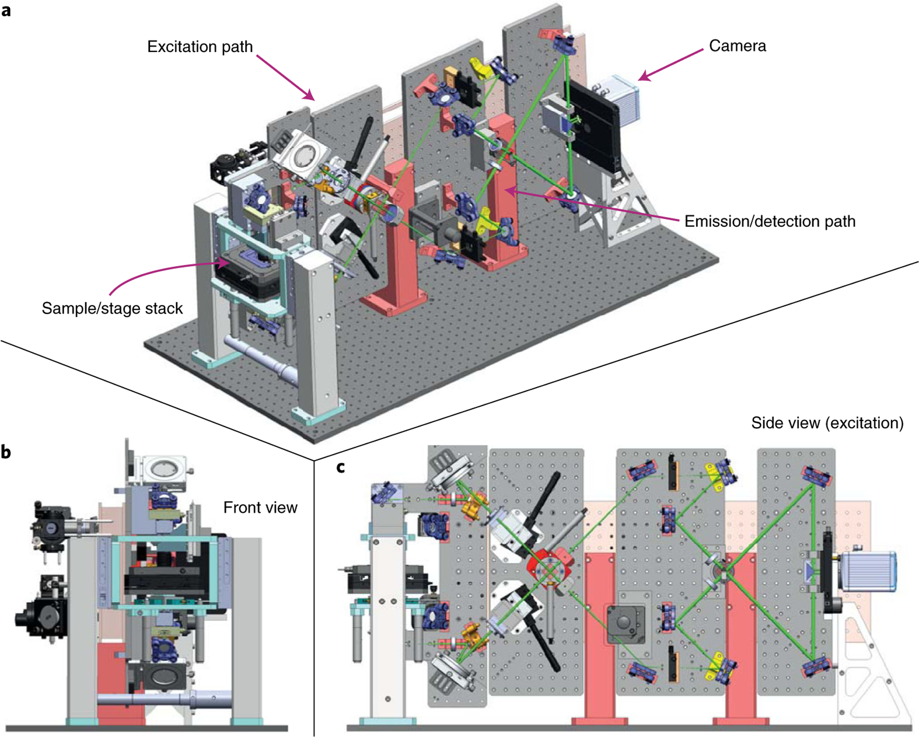
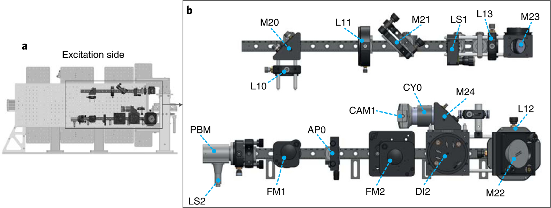
The development of single-molecule switching (SMS) fluorescence microscopy (also called single-molecule localization microscopy) over the last decade has enabled researchers to image cell biological structures at unprecedented resolution. Using two opposing objectives in a so-called 4Pi geometry doubles the available numerical aperture, and coupling this with interferometric detection has demonstrated 3D resolution down to 10 nm over entire cellular volumes. The aim of this protocol is to enable interested researchers to establish 4Pi-SMS super-resolution microscopy in their laboratories. We describe in detail how to assemble the optomechanical components of a 4Pi-SMS instrument, align its optical beampath and test its performance. The protocol further provides instructions on how to prepare test samples of fluorescent beads, operate this instrument to acquire images of whole cells and analyze the raw image data to reconstruct super-resolution 3D data sets. Furthermore, we provide a troubleshooting guide and present examples of anticipated results. An experienced optical instrument builder will require ~12 months from the start of ordering hardware components to acquiring high-quality biological images.

Fig. 1 |. 4Pi-SMS detection and excitation path optical overview.

a, 4Pi-SMS detection light path. Fluorescence emission is collected by two opposing objective lenses (OBJ0 and OBJ1) and then directed into two symmetric, identical upper (blue) and lower (green) beam paths. The respective beam paths traverse broadband achromatic QWPs (QWP0 and QWP1), dichroic mirrors for the introduction of excitation laser light (DI0 and DI1), two lens pairs for imaging the objective back pupil plane onto DMs (DM0 and DM1) and finally meet at a nonpolarizing 50/50 beamsplitter cube (NPBS). The light paths from the two objectives to the NPBS comprise the interference cavity. After the NPBS, the beam paths pass several mirrors and lenses before reaching the camera at the end of the image separation path (red). M, mirror; PBS0, polarizing beam splitter cube; QBF, quadband filter; W, wedge. Emphasis Type=“Bold”>b, 4Pi-SMS illumination light path (red). Light emitted from a fiber (LS2) is collimated (PBM) and follows a straight path through a rectangular aperture (AP0) until it is focused into the back aperture of OBJ1. Alternatively, flip mirrors (FM1 and FM2) direct the beam through a telescope (L10 and L11) to illuminate a large area in the sample (light red). Propagating counter to the illumination path, 940-nm light is launched from a fiber (LS1) and collimated (L13) before passing from OBJ0 to OBJ1 and being separated with a dichroic mirror (DI2), passing a cylindrical lens (CY0) and being focused onto a camera (CAM1) for objective alignment (dashed lines).

Fig. 2 |. 4Pi-SMS system overview.

The different sections of the system are indicated in a, the system is shown from the front, sample side in b and a side view shows the emission/detection path in c.

Fig. 3 |. Detection path beam-alignment tool.

Diagram (a) and a photo (b) of a pinhole alignment tool with a 3-mm 532 laser incident on the target pinhole when installed for alignment. Two alignment tools are used together for alignment of a straight beam path in each segment of the emission beam path (c).

Fig. 4 |. Waveplate orientation and example calibration data.

QWP orientation in the microscope (a) and example wave plate orientation calibration data for both wave plates (b and c).

Fig. 5 |. QWP calibration setup.

a, QWP calibration is begun by directing a vertically polarized alignment laser into a continuously rotating polarizer with photodiode. b, QWP0 is inserted into the beam, and calibration data are collected. c, QWP0 is removed, QWP1 is installed and calibration data are collected. d, Both QWPs are installed to finalize their orientation.

Fig. 6 |. Microscope tower assembly and stage stack.

M6 bolt locations loosened during LS-50 stage installation are indicated with red arrows for the right leg (the same positions for the left leg should also be loosened). An additional location, out of view, in the rear of the tower leg base is indicated with a black arrow. Fine adjustment between the tower legs is made with the telescoping base indicated with the green arrow.

Fig. 7 |. NPBS and wedge assembly.

a, Two registration tabs (raised edges, indicated with arrows) are provided to seat the NBPS cube against before adhering to its mount. b, Before gluing the optical flat and wedge pair, it is helpful to place a lens tissue between the wedge pair to ensure that they are parallel, are not touching and have minimal separation.

Fig. 8 |. DM installation.

a, Overview of inserting a DM into a mount (LP-2A-XYZ, Newport). The front mounting bracket is attached to the opposite side as used here and must be switched. b, The DM installed in the LP-2A mount with the plane for a cross-sectional view (green) shown in c. Ensure that the front retaining ring is installed at the depth shown in c and that the brass housing is flush with the mount body. This ensures that the DM is seated at the correct starting position. d, The orientation of the DM can be observed by inspecting the cable aperture in the back plate.

Fig. 9 |. Alignment laser setup.

An alignment laser (LS0) is launched at two fold mirrors (M0 and M1) and directed through two irises, IR0 and IR1. It reflects from a 45° mirror (M2) to a flip mirror (FM0), where it reflects and enters the interference cavity for alignment.

Fig. 10 |. Labeled diagram of the 4Pi-SMS emission path.

AP1 and AP2, apertures; CAM0, primary imaging sCMOS camera; DI0 and DI1, dichroic beam splitters; DM0 and DM1, deformable mirrors; FW, filter wheel; IR0–14, iris diaphragms; L0–9, lenses; LS0, alignment laser; M0–17, mirrors; OBJ0 and OBJ1, objective lenses; PH0–24, pinhole tool positions (highlighted with red dots) with dowels; QWP0 and QWP1, quarter waveplates; TS0–3, linear actuators; W0 and W1, wedge/flat assemblies.

Fig. 11 |. DM control pattern used for centering.

a, DM control pattern: a 1.25-μm stroke is applied to the center 2 × 2 actuators (yellow). b, An example beam profile recorded on the alignment camera when the alignment laser hits the DM center.

Fig. 12 |. Objective pupil plane location and alignment camera setup.

a, The objective pupil position is 19.1 mm inside the objective measured from the objective shoulder. b, Alignment camera mounted on a compact holder with RMS thread adaptor such that the camera sensor sits at the position of the objective pupil plane relative to the RMS thread shoulder.

Fig. 13 |. DM conjugation.

a, Image of the full DM surface when the camera sensor and DM membrane are not conjugated. b, Zoom-in image of the DM surface when the camera sensor and the DM surface are conjugated (the corresponding region is shown in the purple box in a). When conjugated correctly, the pattern from the DM surface (bright area) can no longer be seen while the fine connection wires and electrodes at the edge of the reflective membrane are in focus (lower portion of b).

Fig. 14 |. Excitation path diagram with labels used throughout the alignment procedure.

AP0, adjustable aperture; CAM1, USB CMOS camera (DCC1545M, Thorlabs); CY0, cylindrical lens; DI2, short-pass dichroic beam splitter (DMSP805L, Thorlabs); FM1 and FM2, flip mirrors; L10–13, achromatic lenses; LS1, 940-nm laser (LP940-SF30, Thorlabs); LS2, fiber from multi-color laser module including both a 642-nm laser and an activation 405-nm laser; M20–24, silver mirrors; PBM, parabolic mirror.

Fig. 15 |. Sample mounting in custom holder FAB-P0035.

a, Exploded view of the sample holder and coverslip assembly. b, Resulting geometry of the sample holder located between two opposing objective lenses for imaging. c, Photo of mounted sample.

Fig. 16 |. Image layout on data-acquisition camera.

Fluorescent bead images on the primary imaging camera arranged in a line along the X-dimension. Two sets of images are visible with a gap between them. Images S2 and P1 are flipped relative to S1 and P2. The scale bar is 5 μm.

Fig. 17 |. Example interference scan data.

Example interference data when scanning a single bead by translating the stage stack through the central interference position.

Fig. 18 |. Interference variation across the field of view.

After initial setup, interference will vary across the ~20 × 20-μm field of view as shown in a when viewed with a high-density bead sample (simulated images). Yellow lines in a guide the eye in seeing the constructive interference fringes. As the OBJ1 and the NPBS are iteratively adjusted, the number of fringes will be reduced as shown in b. After careful adjustment, the interference phase across the field of view can be made reasonably uniform as shown in c.

Fig. 19 |. Example quartz wedge calibration data for setting the phase between the four interference images.

The quartz wedge motor position versus phase for both color channels is shown in a, while the resulting reduced moments for the 600/52 filter and 700/75 filter are shown in b and c, respectively.

Fig. 20 |. Fluorescent bead with and without astigmatism above and below the focal plane.

a, Image of a single fluorescent bead at the focal plane without application of astigmatism. The same fluorescent bead is shown in b with astigmatism applied while in focus and defocused by −600 nm (c) and +600 nm (d), respectively. The scale bar is 1 μm.

Fig. 21 |. Reduced moment versus Z position and phase calibration data example.

a, Reduced moment for the four phase images. b, Unwrapped phase versus sample Z position fit to a linear function.

Fig. 22 |. Objective lock NIR laser focus.

A 940-nm NIR laser is used to track the relative position of the two objective lenses. After passing through OBJ1 and being collected by OBJ0, the beam passes a cylindrical lens and is focused on a camera. When the object’s axis separation changes (defocused) by −1 μm, the NIR laser spot appears as in a on the camera. When the objectives are ‘in focus’, the spot appears as in b, and when they are axially separated by +1 μm, the NIR spot appears as in c. The scale bar is 20 μm.

Fig. 23 |. Example environmental vibration data.

a, Anticorrelated intensity values of the same bead in different images indicate that vibrations lower the axial localization precision of the system. b, The power spectral density visualization of the same recording reveals pronounced frequencies. c, To find vibration sources nearby, it is helpful to plot recorded (audio) spectra as a function of time. Fingerprint-like patterns point to different sources, as seen for distinct patterns around 44 and 49 Hz in this case and 50 Hz (probably linked to the frequency of AC power delivery).

Fig. 24 |. DM surface interference images.

Interferograms for a functional (a) and damaged (b) DM.

Fig. 25 |. Example 4Pi-SMS images from immunostained microtubules and Nup96-SNAP labeled nuclear pore complexes.

a, 4Pi-SMS image of indirectly immunostained ɑ-tubulin labeled with CF660C in a COS7 cell in water-based imaging buffer. b and c, Axial views of the indicated regions in a. d, 4Pi-SMS image of Nup96-SNAP labeled with BG-Alexa 647 in the lower nuclear envelope of a U2OS cell in TDE-based index-matching imaging buffer. e, XZ projection of the indicated region in d. f, Fitting two Gaussians to the axial line profile of an individual nuclear pore complex quantifies the result. Scale bars are 1 μm (a), 100 nm (b,d, and e) and 50 nm (c).

References

1. Shtengel G et al. Interferometric fluorescent super-resolution microscopy resolves 3D cellular ultrastructure. Proc. Natl Acad. Sci. USA 106, 3125–3130 (2009). - PMC - PubMed
1. Aquino D et al. Two-color nanoscopy of three-dimensional volumes by 4Pi detection of stochastically switched fluorophores. Nat. Methods 8, 353–359 (2011). - PubMed
1. Wang G, Hauver J, Thomas Z, Darst SA & Pertsinidis A Single-molecule real-time 3D imaging of the transcription cycle by modulation interferometry. Cell 167, 1839–1852.e21 (2016). - PMC - PubMed
1. Huang F et al. Ultra-high resolution 3D imaging of whole cells. Cell 166, 1028–1040 (2016). - PMC - PubMed
1. Del Viso F et al. Congenital heart disease genetics uncovers context-dependent organization and function of nucleoporins at cilia. Dev. Cell 38, 478–492 (2016). - PMC - PubMed
Publication types