Explaining the effects of distractor statistics in visual search

Abstract

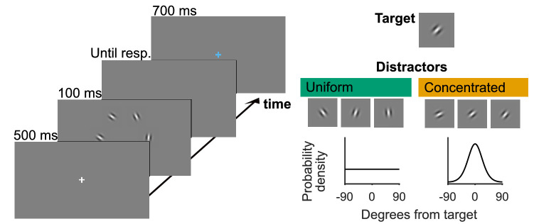
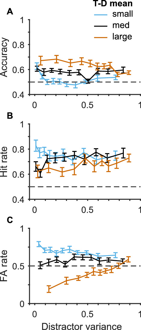
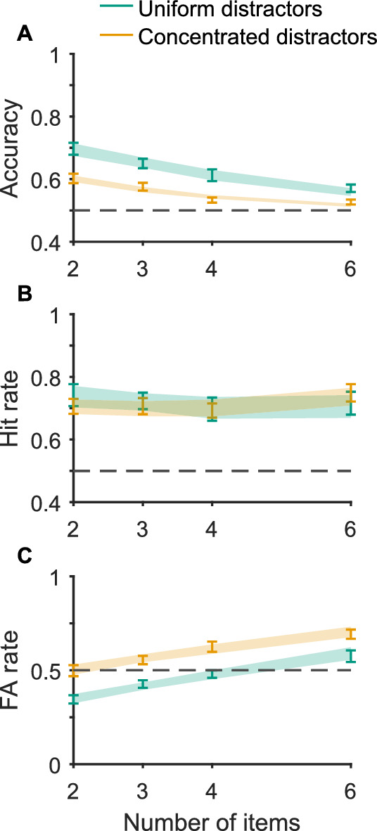
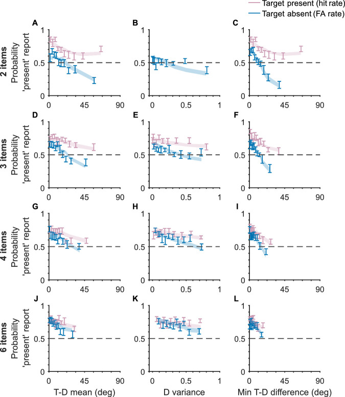
Visual search, the task of detecting or locating target items among distractor items in a visual scene, is an important function for animals and humans. Different theoretical accounts make differing predictions for the effects of distractor statistics. Here we use a task in which we parametrically vary distractor items, allowing for a simultaneously fine-grained and comprehensive study of distractor statistics. We found effects of target-distractor similarity, distractor variability, and an interaction between the two, although the effect of the interaction on performance differed from the one expected. To explain these findings, we constructed computational process models that make trial-by-trial predictions for behavior based on the stimulus presented. These models, including a Bayesian observer model, provided excellent accounts of both the qualitative and quantitative effects of distractor statistics, as well as of the effect of changing the statistics of the environment (in the form of distractors being drawn from a different distribution). We conclude with a broader discussion of the role of computational process models in the understanding of visual search.

Figure 1.

Interaction between target-to-distractor mean difference (T-D mean) and distractor variance on the probability of a confusing distractor (Rosenholtz, 2001). When T-D mean is large, then increasing distractor variance makes a distractor that closely resembles the target more likely. On the other hand, when T-D mean is small, increasing distractor variance actually makes it less likely that there is a distractor that is highly similar to the target.

Figure 2.

Participants performed a visual search task in which they had to report the presence or absence of a target (a Gabor oriented at 45${}^{\circ }$ clockwise from vertical) in a briefly presented display. The display contained between two and six items. There were two distractor environments, one in which all distractor orientations were equally likely and one in which distractor orientations were more likely to be close to the target orientation. The plots of distractor distributions in the two conditions are accurate, while experiment “screenshots” are for illustration and not to scale.

Figure 3.

The distributions of distractor statistics, separately for the cases of two, three, four, and six items in the display (including the target). The area under the curves in all 12 plots is the same. Note that these distributions are determined by stimuli properties and are completely independent of participant behavior. Here and throughout the article, target-to-distractor mean difference (T-D mean) refers to the absolute difference between the circular mean of the distractors and the target orientation, and distractor variance refers to the circular variance of the distractors. Minimum target-distractor difference (min T-D difference) refers to the absolute difference between the target orientation and the distractor closest to this orientation. Data from all participants combined are shown. We can see that distractor statistic distributions are highly nonuniform. This is the motivation for, in all other plots than this one, quantile binning distractor statistics.

Figure 4.

The effect of T-D mean and distractor variance on behavior. There was a particularly clear interaction effect on FA rate, consistent with a signal detection theory account. For the plot, T-D mean was divided into three bins, participant by participant. The average edges between bins were at 12${}^{\circ }$ and 36${}^{\circ }$. Data from trials with three, four, and six items were used for plotting.

Figure 5.

The relationship between the local log-likelihood ratio ($d_i$) and measured orientation ($x_i$). For a range of values ($\kappa =e^1,e^2,e^3$; ${\kappa }_s=0,1.5$), we observed that the local log-likelihood ratio was maximal when the measured orientation matched the target orientation (0) and decreased as measured orientation moved away from this value.

Figure 6.

The effect of all summary statistics when considered individually (error bars) and model fits for these effects (shading). The Bayesian observer model captures the observed effects well.

Figure 7.

Decision thresholds used by the Bayesian observer for the case of two items. Also shown are the shape of the decision thresholds corresponding to a heuristic strategy in which the decision is based on the item closest to the target (see Modeling methods). The axes represent measurements of the items made by the observer, relative to the target orientation. If the measurements fall within the marked area, the observer reports “target present.” The Bayesian observer thresholds were calculated using $\sigma ={10}^{\circ }$ and under a range of values for ${\sigma }_s$, including those used in the experiment (uniform environment, ${\sigma }_s=\infty$; concentrated environment, ${\sigma }_s={29}^{\circ }$). For high ${\sigma }_s$, the Bayesian observer effectively only uses the measurement closest to the target to make their decision.

Figure 8.

Interaction between T-D mean and distractor variance and model fits for these effects. The model captures the interaction of T-D mean and distractor variance on FA rate, along with the trends in accuracy.

Figure 9.

The effect of number of items. The Bayesian observer model captured the reduction in accuracy with more items and the increase in false alarms.

Figure 10.

Effect of distractor statistics in the uniform environment, at different numbers of items. The Bayesian observer model successfully accounts for most effects at all numbers of items considered, although there appear to be some systematic deviations.

Figure 11.

Effect of distractor statistics in the concentrated environment, at different numbers of items. The Bayesian observer model successfully accounts for most effects observed.

Figure 12.

Mean AIC and BIC relative to the best-fitting model and the number of participants best fit by each model. See Table 3 for details of the models. Model comparison results were inconclusive because a consistent pattern of results was not found across AIC and BIC. Unlike in other plots, error bars here reflect 95% bootstrapped confidence intervals.

Figure 13.

Data and Model 2 fits for the effect of distractor variance on FA rate. Model 2 assumes observers ignore the difference between the two distractor environments. Nevertheless, the model can predict differences between the two environments. This is likely because distractor environment correlates with other distractor statistics.

Figure 14.

The individual effect of three distractor statistics on accuracy, hit rate, and FA rate. As the T-D mean and min T-D difference increased, performance also increased and “target present” responses decreased. Surprisingly, distractor variance only had an effect on FA rate.

Figure 15.

The effect of all summary statistics when considered individually (error bars) and Model 3 fits for these effects (shading).

Figure 16.

Interaction between T-D mean and distractor variance.

Figure 17.

The effect of number of items.

Figure 18.

Effect of distractor statistics in the uniform environment, at different numbers of items.

Figure 19.

Effect of distractor statistics in the concentrated environment, at different numbers of items.

Figure 20.

Number of fits out of 40 resulting in a log-likelihood within 1 point of the maximum log-likelihood found. Model numbers refer to Table 3. More saturated colors represent higher success rates. (A) First run. (B) Second run. The differences between the runs are described in the text.

References

1. Acerbi L., Dokka K., Angelaki D. E., & Ma W. J. (2018). Bayesian comparison of explicit and implicit causal inference strategies in multisensory heading perception. PLoS Computational Biology, 14, e1006110, doi:10.1371/journal.pcbi.1006110. - DOI - PMC - PubMed
1. Acerbi L. & Ma W. J. (2017). Practical Bayesian optimization for model fitting with Bayesian adaptive direct search. In Advances in Neural Information Processing Systems 30 (pp. 1836–1846). Retrieved from http://papers.nips.cc/paper/6780-practical-bayesian-optimization-for-mod....
1. Afshartous D. & Preston R. A. (2011). Key results of interaction models with centering. Journal of Statistics Education, 19(3), doi:10.1080/10691898.2011.11889620. - DOI
1. Berens P. (2009). CircStat: A MATLAB toolbox for circular statistics. Journal of Statistical Software, 31(10), 1–21, doi:10.18637/jss.v031.i10. - DOI
1. Bhardwaj M., van den Berg R., Ma W. J., & Josić K. (2016). Do people take stimulus correlations into account in visual search? PLoS ONE, 11(3), 1–16, doi:10.1371/journal.pone.0149402. - DOI - PMC - PubMed
Publication types