scTenifoldNet: A Machine Learning Workflow for Constructing and Comparing Transcriptome-wide Gene Regulatory Networks from Single-Cell Data

Abstract

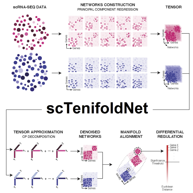
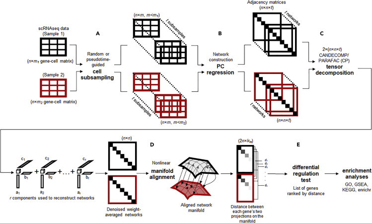
We present scTenifoldNet-a machine learning workflow built upon principal-component regression, low-rank tensor approximation, and manifold alignment-for constructing and comparing single-cell gene regulatory networks (scGRNs) using data from single-cell RNA sequencing. scTenifoldNet reveals regulatory changes in gene expression between samples by comparing the constructed scGRNs. With real data, scTenifoldNet identifies specific gene expression programs associated with different biological processes, providing critical insights into the underlying mechanism of regulatory networks governing cellular transcriptional activities.

Keywords: gene regulatory network; machine learning; manifold alignment; principal-component regression; scRNA-seq; scTenifoldNet; single-cell RNA sequencing; tensor decomposition.

Graphical abstract

Figure 1

Overview of the scTenifoldNet Workflow scTenifoldNet is a machine learning framework that uses a comparative network approach with scRNA-seq data to identify regulatory changes between samples. scTenifoldNet is composed of five major steps. (A) Cell subsampling. scTenifoldNet starts with subsampling cells in the scRNA-seq expression matrices. When two samples are analyzed, each of the two samples is subsampled either randomly or following a pseudotime trajectory of cells. The subsampling is repeated multiple times to create a series of subsampled cell populations, which are subject to network construction and form a multilayer scGRN. (B) Network construction. PC regression is used for scGRN construction; each scGRN is represented as a weighted adjacency matrix. (C) Tensor denoising. Two samples produce two multilayer GRNs and form two three-order tensors, which are subsequently decomposed into multiple components. The top components of tensor decomposition are then used to reconstruct two denoised multilayer scGRNs. Then, two denoised multilayer scGRNs are collapsed by taking the average weight across layers. (D) Manifold alignment. The two single-layer average scGRNs are then aligned with respect to common genes using a nonlinear manifold alignment algorithm. Each gene is projected to a low-rank manifold space as two data points, one from each sample. (E) Differential regulation test. The distance between the two data points is the relative difference of the gene in its regulatory relationships in the two scGRNs. Ranked genes are subject to tests for their significance in differential regulation between scGRNs.

Figure 2

Benchmarking the Performance of scTenifoldNet Using Simulated Data (A) The accuracy and recall of scGRN construction using different methods, PC regression, SCC, MI, and GENIE3, as functions of the number of cells used in the analysis. Error bar is the SD of the computed values after 10 bootstrapped evaluations. PCR, PC regression; SCC, Spearman’s correlation coefficient; MI, mutual information; GENIE3, a random-forest-based network construction method. (B) Visualization of the effect of tensor denoising on accuracy and recall of multilayer scGRNs. Each subpanel is a heatmap of a 100 × 100 adjacency matrix constructed using PC regression over the counts of 500 randomly subsampled cells. Gray scale indicates the relative strength of regulatory relationships between genes. Top part includes networks before tensor denoising (adjacency matrices in heatmap with red box); bottom part includes corresponding networks after tensor denoising (adjacency matrices in heatmap with green box). In each part, adjacency matrices of networks of 10 subsamples (10 small heatmaps) and their average adjacency matrix (one large heatmap) are shown. (C) Evaluation of the sensitivity of scTenifoldNet in identifying punctual changes in the regulatory profiles. Top: evaluation of the original data matrix against itself. Bottom: evaluation of the original matrix against the perturbed matrix. Significant genes identified using the differential regulation test (FDR <0.1, B-H correction) are indicated in red. All significant genes are perturbed in simulation and thus are expected to be identified.

Figure 3

Analysis of Transcriptional Responses to Morphine in Mouse Cortical Neurons (A) Illustration of experimental design and data collection of the morphine response study. (B) t-SNE plot of 7,972 and 8,912 neurons from morphine-treated (blue) and mock-treated (red) mice, respectively. (C) Violin plots showing the log-normalized expression levels of representative differentially regulated and/or differentially expressed genes in four (M) morphine- and four (C) mock-treated mice. (D) Quantile-quantile (Q-Q) plot for observed and expected p values of the 8,138 genes tested. Genes (n = 65) with FDR <0.1 are shown in red; genes (n = 56) with FDR <0.05 are labeled with an asterisk. Inset shows results of the GSEA for genes ranked by their distances in manifold aligned scGRNs from morphine- and mock-treated mice. (E) The module enriched with differentially regulated genes and the corresponding subnetworks in two scGRNs. For illustrative purposes, the module is centered on the differentially regulated gene Ppp3ca. Significantly differentially regulated genes (FDR <0.05) in the module are highlighted in green. Edges are color-coded: red indicates a positive association, and blue indicates negative. Weak edges are filtered out by thresholding for clear visualization, and the background shadow indicates the shared portion of the module in the two scGRNs.

Figure 4

Analysis of Transcriptional Responses of a Carcinoma Cell Line to Cetuximab (A) Illustration of experimental design, including sample groups and the known mechanism of drug action, in the study of cetuximab resistance of HNSCC cell lines. (B) t-SNE plot of 5,217 and 4,507 HNSCC-SCC6 cells treated with cetuximab (red) and PBS (blue), respectively. (C) Violin plots showing the log-normalized expression levels of selected differentially regulated genes in SCC6 cells with and without cetuximab treatment. (D) Q-Q plot for observed and expected p values of the 7,503 genes tested. Genes (n = 25) with FDR <0.05 are labeled with an asterisk. Inset shows the results of the GSEA for genes ranked by their distances in manifold aligned scGRNs from young and old mice. (E) A representative module with differentially regulated genes and corresponding subnetworks in two scGRNs. The module is enriched with differentially regulated genes and the corresponding subnetworks in two scGRNs. For illustrative purposes, the module is centered on the differentially regulated gene H2AFZ. The colors, edges, and marks are presented as in Figure 3E.

Figure 5

Analysis of Transcriptional Responses of Alveolar Type 1 Cells to Nkx2-1 Gene Knockout (A) Illustration of experimental design and data collection of the KO experiment. (B) t-SNE plot of 2,397 and 638 AT1 cells from Nkx2-1 KO mice (red) and WT mice (blue). (C) Violin plots showing the log-normalized expression levels of selected differentially regulated genes in KO (red) and WT (blue) mice. (D) Q-Q plot for observed and expected p values of tested genes. Genes (n = 29) with FDR <0.05 are labeled with an asterisk. Inset shows the results of GSEA for genes ranked by their distances in manifold aligned scGRNs. (E) A representative module that contains the differentially regulated gene Tpt1 in the WT mice. Most parts of the module disappear in the KO mice. The colors, edges, and marks are presented as in Figure 3E.

Figure 6

Analysis of Transcriptional Responses of Human Dermal Fibroblasts to a Double-Stranded RNA Stimulus (A) Illustration of experimental design and tested mechanism of transcriptional responses. (B) t-SNE plot of human dermal fibroblasts before (blue) and after (red) dsRNA stimulus. (C) Violin plots showing the log-normalized expression levels of selected differentially regulated genes before (blue) and after (red) stimulus. (D) Q-Q plot for observed and expected p values of tested genes. Genes (n = 29) with FDR <0.05 are labeled with an asterisk. Inset shows the results of GSEA for genes ranked by their distances in manifold aligned scGRNs. (E) Comparison of a representative module that contains three differentially regulated genes in the control sample. The colors, edges, and marks are presented as in Figure 3E. (F) Scatterplots showing the correlation between TPT1 and ANXA2 before (top) and after (bottom) dsRNA stimulus.

Figure 7

Analysis of Transcriptional Responses of Neurons to Aβ Peptides in 5xFAD Mice, a Model of Alzheimer Disease (A) Illustration of experimental design and data collection of the 5xFAD mouse study. (B) t-SNE plot of neurons of the 5xFAD (red) and WT (blue) mice. (C) Violin plots showing the log-normalized expression levels of selected differentially regulated genes in neurons of the 5xFAD (red) and WT (blue) mice. (D) Q-Q plot for observed and expected p values of tested genes. Genes (n = 18) with FDR <0.05 are labeled with an asterisk. Inset shows the results of the GSEA for genes ranked by their distances in manifold aligned scGRNs. (E) Comparison of a representative module that contains top-ranked differentially regulated genes between the two scGRNs. The colors, edges, and marks are presented as in Figure 3E.

References

1. Margolin A.A., Nemenman I., Basso K., Wiggins C., Stolovitzky G., Dalla Favera R., Califano A. ARACNE: an algorithm for the reconstruction of gene regulatory networks in a mammalian cellular context. BMC Bioinformatics. 2006;7(Suppl 1):S7. - PMC - PubMed
1. Huynh-Thu V.A., Irrthum A., Wehenkel L., Geurts P. Inferring regulatory networks from expression data using tree-based methods. PLoS One. 2010;5 doi: 10.1371/journal.pone.0012776. - DOI - PMC - PubMed
1. Marbach D., Costello J.C., Kuffner R., Vega N.M., Prill R.J., Camacho D.M., Allison K.R., Consortium D., Kellis M., Collins J.J. Wisdom of crowds for robust gene network inference. Nat. Methods. 2012;9:796–804. - PMC - PubMed
1. Friedman N., Linial M., Nachman I., Pe'er D. Using Bayesian networks to analyze expression data. J. Comput. Biol. 2000;7:601–620. - PubMed
1. Gill R., Datta S., Datta S. A statistical framework for differential network analysis from microarray data. BMC Bioinformatics. 2010;11:95. - PMC - PubMed
LinkOut - more resources