Continuous Whole-Body 3D Kinematic Recordings across the Rodent Behavioral Repertoire

Abstract

In mammalian animal models, high-resolution kinematic tracking is restricted to brief sessions in constrained environments, limiting our ability to probe naturalistic behaviors and their neural underpinnings. To address this, we developed CAPTURE (Continuous Appendicular and Postural Tracking Using Retroreflector Embedding), a behavioral monitoring system that combines motion capture and deep learning to continuously track the 3D kinematics of a rat's head, trunk, and limbs for week-long timescales in freely behaving animals. CAPTURE realizes 10- to 100-fold gains in precision and robustness compared with existing convolutional network approaches to behavioral tracking. We demonstrate CAPTURE's ability to comprehensively profile the kinematics and sequential organization of natural rodent behavior, its variation across individuals, and its perturbation by drugs and disease, including identifying perseverative grooming states in a rat model of fragile X syndrome. CAPTURE significantly expands the range of behaviors and contexts that can be quantitatively investigated, opening the door to a new understanding of natural behavior and its neural basis.

Keywords: animal tracking; autism; behavior; computational ethology; grooming; individuality; motion capture; phenotyping.

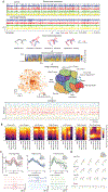
Figure 1 ∣. CAPTURE: Continuous Appendicular and Postural Tracking Using Retroreflector Embedding.

(A) Schematic of the CAPTURE apparatus. Twelve motion capture cameras continuously track the position of 20 body piercings affixed to the animal’s head, trunk, and limbs. (B) Upper: Schematic depictions of a rat with attached markers, colored by the major body segments tracked, engaging in different species-typical behaviors. Lower: hypothetical wireframe representation of 3D marker positions tracked by motion capture for each of the depicted behaviors. (C) Speed of markers located on a single rat’s head, trunk, and appendages, across 72 hours of near-continuous motion capture recordings (upper), measured alongside the speed of the animal’s center-of-mass and the state of the room lights (‘on’ or ‘off’). Investigation of kinematics on minute-long timescales (lower) reveals modulation into alternating periods of movement and rest. Speed traces smoothed with a 30-s boxcar filter. (D) During a behavioral sequence of scratching, rearing, and walking (upper), CAPTURE recordings reveal rhythmic modulation of a selected subset of body part Cartesian and joint angle velocity components (middle). Visualization of individual behaviors on millisecond timescales shows independent control of different appendages during scratching and wet dog shake behaviors (lower). We defined joint angles with respect to sagittal (s), coronal (c), transverse (t), and inter-segment planes (i)(Methods). Shaded regions in C and D denote expanded regions in lower panels. See also Figures S1-S3, Videos S1-S3, Table S1, Methods S1-S2.

Figure 2 ∣. 2D Convolutional networks are ill-suited for whole-body 3D tracking across multiple behaviors.

(A–B) Example video images, as well as wireframe representations of the tracked points for tracking using CAPTURE and DeepLabCut. We trained DeepLabCut using between 100 and 100,000 video frames with labels indicating the position of the 20 marker sites tracked using CAPTURE. DeepLabCut predictions were made using 6 cameras for animals bearing markers in (A) or out of (B) the training dataset. (C) The average 3D distance between DeepLabCut predictions and the position of points tracked using CAPTURE, across training frames, camera numbers and the presence of the rat in or out of the training dataset (marked as in-sample or out-of-sample, respectively). The motion capture reprojection error is shown for comparison. Errors bars (mean ± s.e.m.) are within markers and computed over 306,356 and 249,241 frames for 3 in-sample and 2 out-of-sample animals, respectively. (D) The 10–30 mm differences in precision between CAPTURE and DeepLabCut can produce dramatic changes in the ability to accurately reconstruct an animal’s pose. We computed the fraction of frames in which the length of 19 different body segments, as reported by DeepLabCut, were within 18 mm of the true segment lengths tracked using CAPTURE, for animals in- and out-of-sample. The fraction of correct segment lengths for CAPTURE is shown for comparison. Shaded error bars (within lines) show standard deviation of 100 bootstrapped samples of frames. See also Figure S4, Video S4, Table S2.

Figure 3 ∣. Comprehensive kinematic profiling of the rat behavioral repertoire.

(A) We developed a behavioral mapping procedure to identify behaviors in CAPTURE recordings. We first defined a set of 140 per-frame features describing the pose and kinematics of rats within a 500 ms local window. Many of these features were obtained by computing the eigenpostures of the rats from the measured kinematics (upper), which consisted of commonly observed postural changes such as rearing or turning to the left and right. We then computed time-frequency decompositions of the eigenposture scores over time using a wavelet transform (middle). We subsampled features from all 16 rats recorded (1.047 billion frames) and co-embedded them in two dimensions using t-SNE to create a behavioral map that we clustered using a watershed transform (Figure S5) (Methods). We annotated clusters in the behavioral map, which showed that behavioral categories segregated to different regions of the map. From these behavioral clusters we then computed ethograms describing behavioral usage over time (lower). (B) The power spectrum of the speed of markers on different body segments during rhythmic behaviors. Because different body segments show large variance in overall power, power spectral densities are separately scaled within each marker group on the head, forelimbs, and hindlimbs. Power spectra computed from n=4 animals on two days. (C) Upper: Power spectral densities of individual behavioral clusters belonging to rhythmic behaviors for one rat over two days. Power spectral densities were computed over the speed of one marker on the body segment listed. Colored lines correspond to examples below. Insets show position of the example behavioral clusters within the coarse behavioral category. Spectral densities are reported relative to 1 (mm·s⁻¹)²/ Hz. Lower: individual instances of marker kinematics randomly drawn from example clusters. (D) Example poses selected from non-rhythmic behavior clusters associated with rearing and stretching. See also Figure S5. Videos S5-S7.

Figure 4 ∣. Rat behavior is hierarchically organized into behavioral sequences and states.

(A) We developed a temporal pattern matching algorithm to detect repeated behavioral patterns in our behavioral recordings. We smooth ethograms over 15-s or 2-minute timescales and compute the pairwise correlation to yield a similarity matrix, which we threshold to extract high-value off-diagonal elements. These correspond to patterns of behavioral usage observed at two or more timepoints in the dataset. We cluster these patterns to identify repeated sequences and states, which can be organized to identify hierarchical structure. Ethograms and similarity matrices are shown from a full day of recording in a one animal smoothed with 4-s and 15-s boxcar filters, respectively. Dendrograms and clustered states are schematic examples. Behaviors colored following Figure 3A. (B) Ethograms, smoothed with a 4-s filter for visualization, shown on minute- (upper) and hour-long (lower) timescales. Ethograms are shown for the subset of behaviors observed during each time period, sorted and shaded by their membership in different behavioral sequences (upper) and states (lower). States and sequences detected using the pattern matching algorithm are shown above and ordered in (B) and (C) by their membership in different behavioral categories. (C) Heatmaps showing the composition of sequences (upper) and states (lower) in terms of different behavioral categories. (D) Examples of behavioral patterning during different sequences and states. Sequences show repeated temporal patterns of behavioral usage while states show average increases in behavioral frequency but without detailed temporal structure. For clarity, only a subset of frequently occurring behaviors are shown. Behaviors are colored by their membership in behavioraI categories as in Figure 3A. (E) To display the hierarchical organization of these sequences and states, we computed a stacked tree, whose lower links reflect the probability of observing different behaviors during each sequence and whose upper links reflect the probability of observing different sequences in each state. Behaviors and links are colored according to their behavioral type: green (grooming): grooming and scratching; blue (idling): prone still and postural adjustment; red (active): investigatory, walking, shaking, and rearing. For clarity, one in eight behaviors are shown, and we only visualize links showing probabilities of occurrence greater than 0.05 and 0.1 for behaviors and sequences, respectively. Shaded region corresponds to region highlighted in (F). (F) Hierarchical arrangement of the right grooming behavioral sequences highlighted in (E; left), as well as example ethograms of a subset of behaviors in each sequence (right). For clarity, in the hierarchy we show only one in four behaviors, and a subset of behavioral states used. Across animals, there was significant mutual information between behavioral state and the grooming sequence observed (0.62 vs 10⁻³ nats, P=0.004, sign test, over 9 days where grooming sequences were observed). Example performance data in B–F shown for a single animal on one full day of recording. Example states and sequences numbered in parenthesis reference behavioral usages shown in C. See also Figure S6-S7, Videos S8-S9.

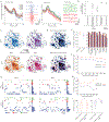
Figure 5 ∣. Caffeine and amphetamine show similar effects on arousal, but divergent effects on behavioral organization.

(A) Behavioral density maps during baseline and after acute administration of either a saline vehicle, caffeine (10 mg/kg) or amphetamine (0.5 mg/kg). The fraction of time animals spent moving compared to baseline (32±1%) increased significantly after administration of caffeine (80±1%) and amphetamine (84±1%) but not after a saline vehicle (17±1%; P=0.016 for caffeine and amphetamine, P=0.4 for vehicle, n=4 rats for drug and vehicle conditions and n=5 rats for baseline condition, 4,635–7,391 s per condition). Both stimulant compounds altered the amount of time spent engaging in walking and rearing (arrows). (B) Caffeine and amphetamine increased the fraction of time spent in active locomotor behaviors at the expense of idling behaviors, but had divergent effects on grooming, with amphetamine alone showing suppression of grooming activity (all P<10⁻⁵, binomial test, n=238-989 effective samples per behavioral category). (C) Caffeine and amphetamine introduced new types of active and grooming behaviors that were rarely observed at baseline, for instance high velocity walks and more vigorous grooming. Colored bars denote fold change significantly modulated behaviors (P<10⁻⁶, Poisson probability of rates in the perturbed condition, Benjamini-Hochberg corrected). Sorting all behavioral changes by their modulation after administration of caffeine (right), reveals that caffeine and amphetamine both increase the frequency of many active behaviors and decrease the frequency of many grooming behaviors. (D) Box-and-whisker plots showing the correlation coefficient of sequence (upper) and state (lower) probability vectors across baseline and drug conditions. Amphetamine and caffeine induced significant changes in the long-timescale organization of behavior (**P=1.5·10⁶, *P<0.005; rank-sum test; n=16 pairs of days between conditions). Because of the lack of movement during vehicle and time-matched controls, baseline data here is taken from two days of recordings. (E) Heatmaps showing the composition of states in terms of behavioral categories (upper) and the fold change in the usage of these states compared to baseline (lower), sorted to emphasize changes across conditions. Amphetamine introduced highly distinct states in animals, emphasized by black lines (Video S10). See also Video S10.

Figure 6 ∣. Fmr1-KO rats show idiosyncratic perseverative body grooming sequences.

(A) Behavioral density maps of Fmr1-WT (n=3) and Fmr1-KO (n=4) age-matched cage mates for two full days of recording. Arrows highlight periods of increased grooming in Fmr1-KO rats. Both wildtype and knockout rats spent equal amounts of time moving (35.1±2% vs 35.0±0.7%, rank-sum test, P=0.85; n=6,8 days of recording in WT and KO rats respectively, 445,601-673,473 s per condition). (B) Fmr1-KO but not Fmr1-WT animals spent increased time grooming, at the expense of idling behaviors (all P<10⁻⁵, binomial test, n_eff=166–232 effective samples per behavioral category). This was accompanied by a significant increase in the dwell time of grooming behaviors alone (10±2% increase in dwell time between KO and WT animals over all grooming behaviors, P=0.03 signed-rank test, n=208 grooming behaviors, compared to <0.01% changes in the average dwell time of active and idling behaviors). (C) The composition of behavioral categories, especially grooming behaviors, were substantially modified in Fmr1-KO but not Fmr1-WT animals. Colored bars denote fold change of behaviors significantly modulated across the stated conditions (P<10⁻⁶, Poisson probability of altered rates, Benjamini-Hochberg corrected). Sorting all behavioral changes by their modulation in Fmr1-KO animals (right), shows little commonality between behaviors modulated in wildtype and knockout animals. (D) Box-and-whisker plots showing the correlation of sequence and state usage probabilities for WT and Fmr1-KO rats. There was a significantly decreased correlation across genotypes (*P=0.0006, P=0.01 for sequences and states, respectively; rank-sum test, n=48 pairs of days between conditions). (E) Heatmaps showing the composition of sequences in terms of behavioral categories (upper) and the fold change in the usage of these sequences compared to baseline (lower), sorted to emphasize changes across conditions. Black lines highlight elevated levels of idiosyncratic grooming sequences in knockout rats.

Figure 7 ∣. Long-timescale behavioral structure is a locus of behavioral individuality.

(A) Left: power spectral densities of the velocity of the front head marker, for two individual behavioral clusters, for n=5 rats over 3-5 days each. Spectral densities are reported relative to 1 (mm·s⁻¹)²/ Hz. Right: the average Cartesian velocity of the head in each behavioral cluster, shown for two rats on three days. Shaded bars are s.e.m. (B) Box plots showing the Pearson correlation of the 140-dimensional behavioral feature vector for five separate comparisons: within-animal, within-day comparisons of (1) different instances of the same behavior, different behaviors in the same coarse category (2) or different behaviors in different coarse categories (3), and of behavioral averages across different days within (4) and across (5) animals. All P<10⁻¹⁰, Kruskal-Wallis test with Bonferroni corrected post-hoc testing, n=1731, 13386, 135094, 5264, 22934, pairs of feature vectors for each comparison, respectively. Only behaviors with at least 5 instances per day were analyzed. (C) Representative behavioral density maps showing consistency of behavior usage from day-to-day for two rats. (D) Overlaid t-SNE density maps across days (upper) and rats (lower). (E) The Pearson correlation between the probability vectors of behavior usage over days, across all categories (left) and per behavioral category (right), over different days and rats. There was a significant decrease in correlation across rats, especially for rearing and grooming behaviors (signed-rank test, P<10⁻⁷ for all comparisons; n=36 and 348 pairs of days within and across animals, respectively). There was a significant correlation between the behavioral usage change over days, and the number of calendar days between recordings (P = 0.002, F-test compared to null model, R² =0.23, n=36), indicating that there was some drift in behavioral usage over time. (F) The Pearson correlation between the probability vectors of behavior usage over days, across 7 increasingly fine-grained clusterings of the behavioral space (Methods). (G) Example ethograms of sequence usage for two rats on two different days, as well as summary bar graphs showing the average sequence usage over the entire day. For clarity, we show only a subset of sequences, smoothed with a 10-s filter. Scale bar on bar plots corresponds to 10% of frames. (H) The average Pearson correlation in the usage of temporal patterns across timescales. We found significantly greater similarity in usage across animals at short timescales compared to long timescales (signed-rank test, P<10⁻¹⁰, 174 pairs of days). (I) We trained a random forest classifier to distinguish individual rats or individual days using behavioral usage statistics. Incorporating long-timescale pattern usage significantly improved identification of species, but not across days within species (signed-rank test, P=0.01, 0.6, respectively, n=21 days). See also Figure S7.

References

1. Agarwal A, and Triggs B (2004). Tracking Articulated Motion Using a Mixture of Autoregressive Models In Computer Vision - ECCV 2004, Pajdla T, and Matas J, eds. (Berlin, Heidelberg: Springer Berlin Heidelberg; ), pp. 54–65.
1. Alahi A, Goel K, Ramanathan V, Robicquet A, Fei-Fei L, and Savarese S (2016). Social lstm: Human trajectory prediction in crowded spaces. In Proceedings of the IEEE Conference on Computer Vision and Pattern Recognition, pp. 961–971.
1. Anderson DJ, and Adolphs R (2014). A framework for studying emotions across species. Cell 157, 187–200. - PMC - PubMed
1. Anderson DJ, and Perona P (2014). Toward a science of computational ethology. Neuron 84, 18–31. - PubMed
1. Angel E (2009). The piercing bible : the definitive guide to safe body piercing (Berkeley, Calif: Celestial Arts; ).
Publication types
LinkOut - more resources