Tracking collective cell motion by topological data analysis

Abstract

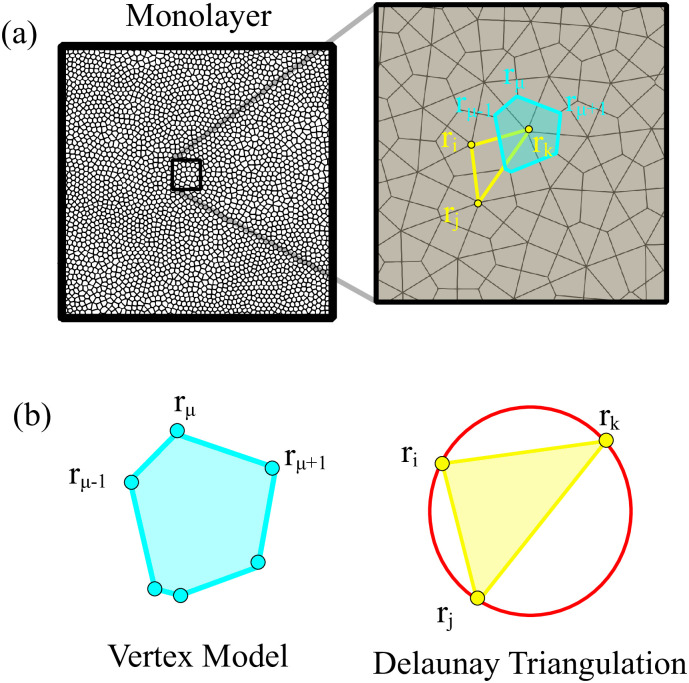
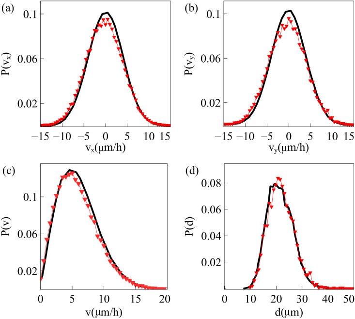
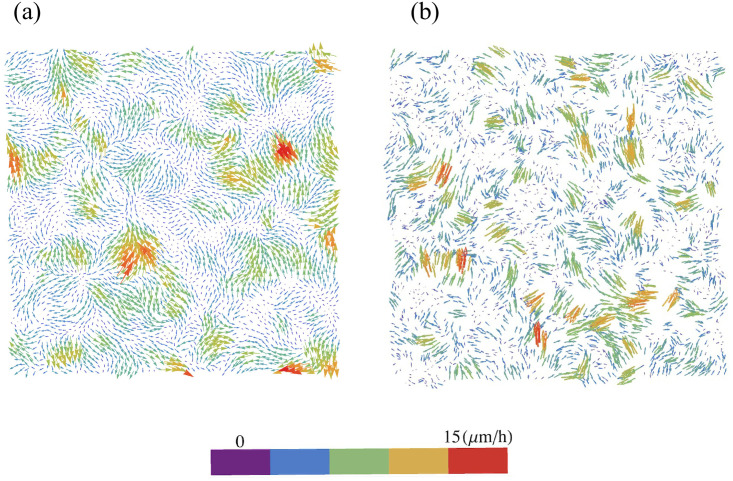
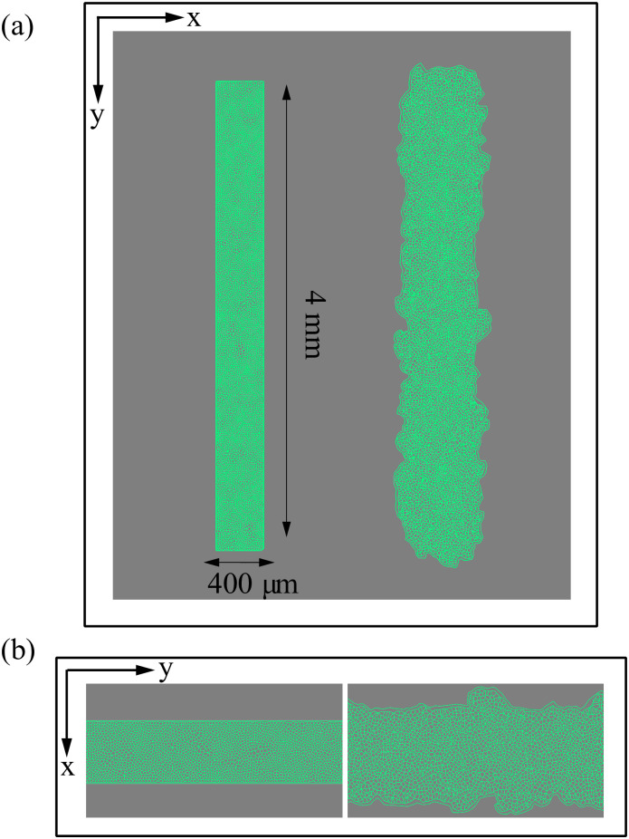
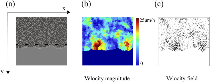
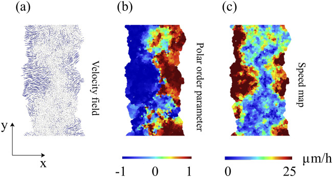
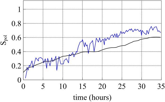
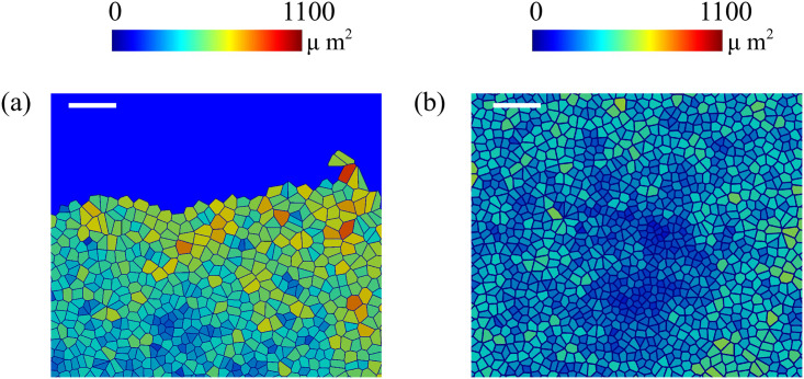
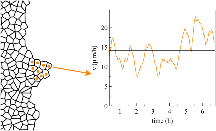
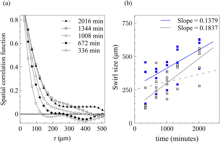
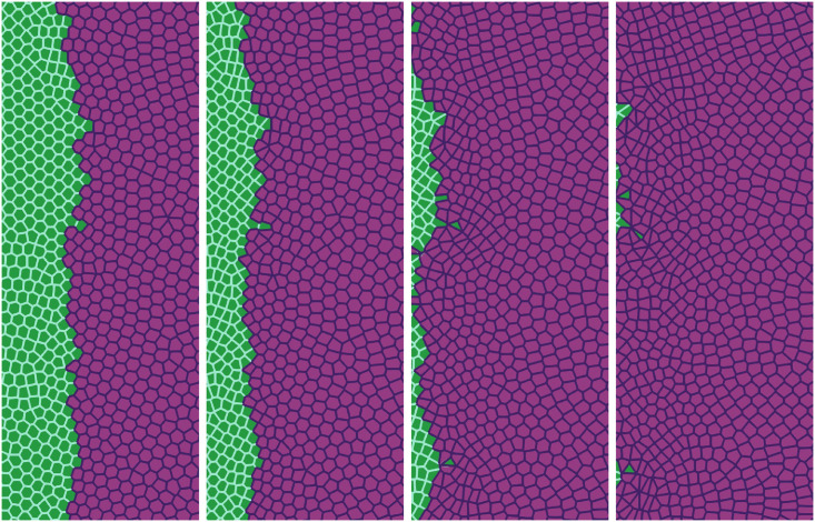
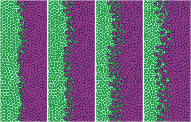
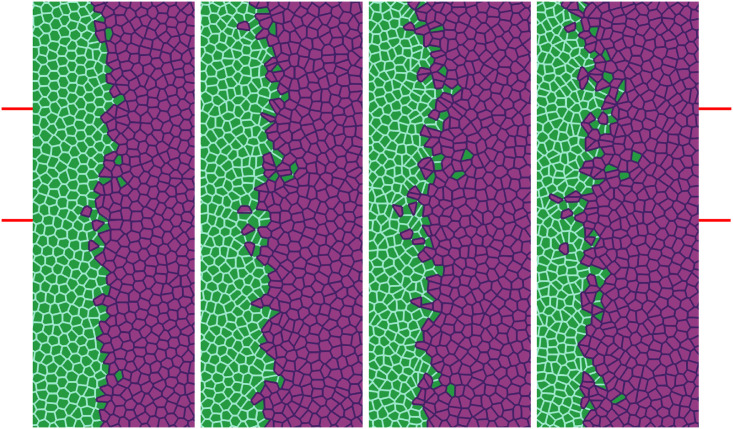
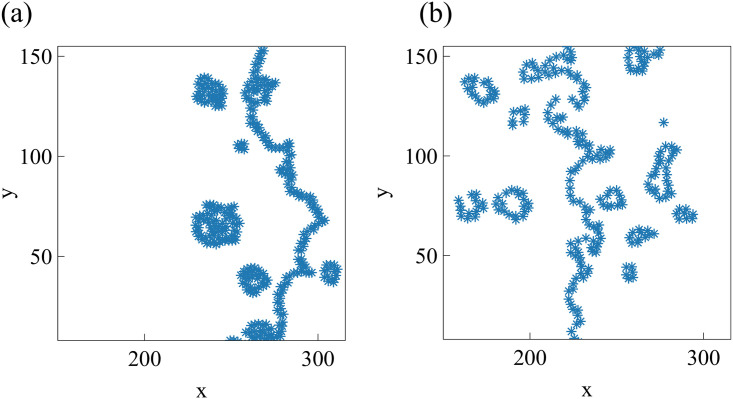
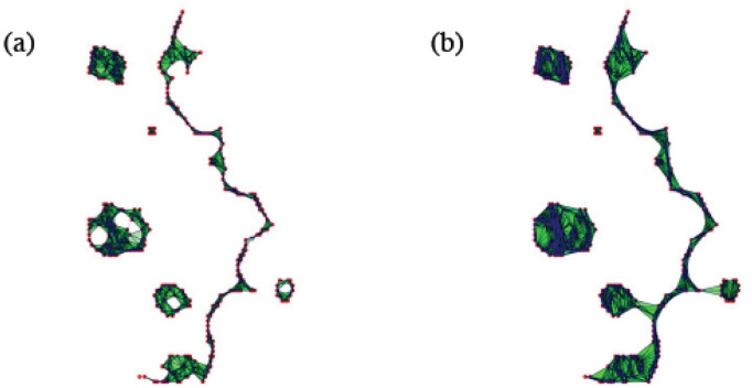
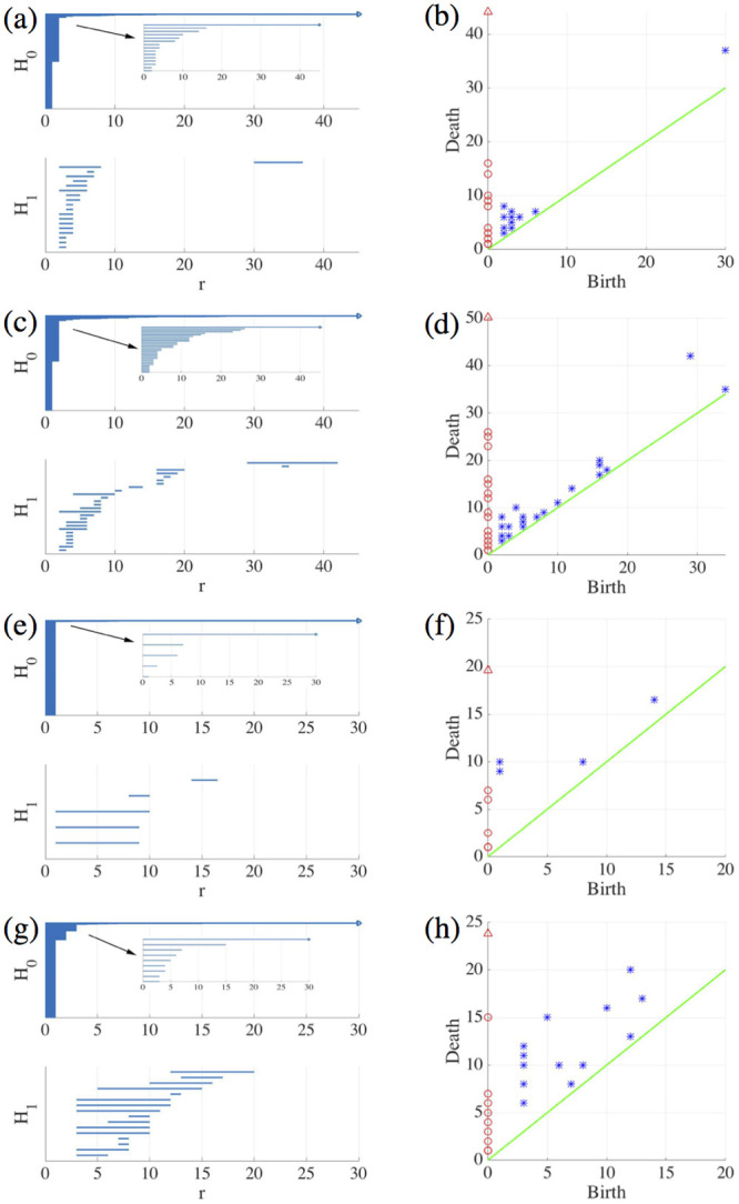
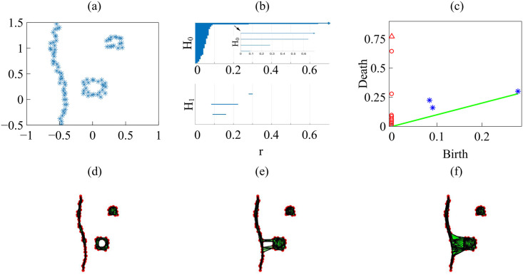
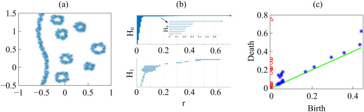
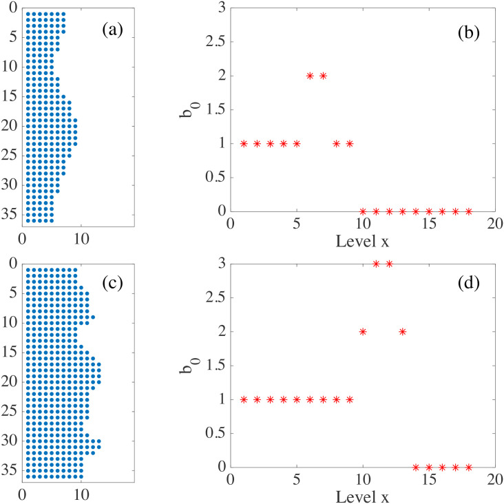
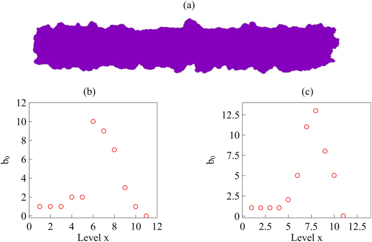
By modifying and calibrating an active vertex model to experiments, we have simulated numerically a confluent cellular monolayer spreading on an empty space and the collision of two monolayers of different cells in an antagonistic migration assay. Cells are subject to inertial forces and to active forces that try to align their velocities with those of neighboring ones. In agreement with experiments in the literature, the spreading test exhibits formation of fingers in the moving interfaces, there appear swirls in the velocity field, and the polar order parameter and the correlation and swirl lengths increase with time. Numerical simulations show that cells inside the tissue have smaller area than those at the interface, which has been observed in recent experiments. In the antagonistic migration assay, a population of fluidlike Ras cells invades a population of wild type solidlike cells having shape parameters above and below the geometric critical value, respectively. Cell mixing or segregation depends on the junction tensions between different cells. We reproduce the experimentally observed antagonistic migration assays by assuming that a fraction of cells favor mixing, the others segregation, and that these cells are randomly distributed in space. To characterize and compare the structure of interfaces between cell types or of interfaces of spreading cellular monolayers in an automatic manner, we apply topological data analysis to experimental data and to results of our numerical simulations. We use time series of data generated by numerical simulations to automatically group, track and classify the advancing interfaces of cellular aggregates by means of bottleneck or Wasserstein distances of persistent homologies. These techniques of topological data analysis are scalable and could be used in studies involving large amounts of data. Besides applications to wound healing and metastatic cancer, these studies are relevant for tissue engineering, biological effects of materials, tissue and organ regeneration.

Fig 1. Voronoi tessellation and Delaunay triangulation.

(a) Here r_μ are vertices of polygons in the Voronoi tessselation and r_i are centers of polygons that are vertices of Delaunay triangles. Here the zoom of a monolayer shows (b) the Voronoi tesselation and the Delaunay triangulation.

Fig 2. Probability distribution function (PDF) for particle velocities: (a) v_x, (b) v_y, (c) v = |v|; and (d) mean distance d between neighboring particles; after the initialization procedure (red triangles) as compared to the experimentally observed PDF (black line) [16].

Parameter values are those in Table 1.

Fig 3. Velocity field obtained from (a) experiments [16], (b) simulations after the initialization procedure.

Parameter values are those in Table 1.

Fig 4. Initial configuration and configuration after 20 h of stencil removal showing the formation of fingers according to the numerical simulation of the model.

(a) Full view, (b) zoom. Initial box size is 1.6 mm², P⁰ = 10, A⁰ = π, and shape index p⁰ = 5.65. Parameter values are those in Table 1. See S1 Video.

Fig 5. Cell velocity field after 2 h of stencil removal in an invasion configuration calculated from simulations of the model with the parameters of Fig 4 and Table 1.

(a) Phase contrast visualizing cells, (b) profile of cell speed (modulus of velocity), (c) velocity field. These panels should be compared with those obtained from experimental MDCK data in Fig 2A of Ref. [10].

Fig 6. (a) Numerically simulated cell velocity field, (b) local polar order parameter cosϑ_i, and (c) speed (|v|) map after 35 h of stencil removal in an invasion configuration for a 400 μm wide strip.

Parameter values as in Fig 5. See S2 Video.

Fig 7. Evolution of the polar order parameter S_pol(t) corresponding to Fig 5.

Here t = 0 corresponds to 1.5 h after stencil removal [10]. An average over 5 simulations exhibits the same trend as measurements reported in Ref. [10] (jagged line).

Fig 8. Areas of cells during a simulation of a spreading configuration: (a) Area of cells near the interface, (b) area of cells far from the interface.

Our simulations exhibit the same trend as measurements reported in Ref. [44]. The bar length in both panels is 100 μm.

Fig 9. Average velocity of the marked cells during finger expansion.

The velocity of each cell oscillates in a similar but somewhat more irregular manner (not shown).

Fig 10

(a) Spatial correlation function I(r, t) corresponding to Fig 6(a) for different times. (b) Correlation length given by the first zero of I(r) (empty squares) and swirl size given by the first local minimum of I(r) (blue squares). Dashed line from swirl sizes in Ref. [11].

Fig 11. Simulation of the antagonistic migration assay: One population advances pushing back the other.

Junction tensions are Λ₁₁ = −6.2, Λ₂₂ = −6.8, which yield shape indices 3.50 (green cells) and 3.84 (magenta cells), respectively. Other parameters are listed in the first row of Table 2, and ${\Lambda }_{12}=-7.0<\frac{1}{2}({\Lambda }_{11}+{\Lambda }_{22})$ correspond to weak population mixing. Snapshots are taken at times 2 h, 6.5 h, 13 h, 20 h. See S3 Video.

Fig 12. Simulation of the antagonistic migration assay: Creation of a extremely rugged interface.

First and second snapshots: ${\Lambda }_{12}=-7.5<\frac{1}{2}({\Lambda }_{11}+{\Lambda }_{22})$ (population mixing); third and fourth snapshots: ${\Lambda }_{12}=-6.0>\frac{1}{2}({\Lambda }_{11}+{\Lambda }_{22})$ (population segregation). Other parameters are listed in the second row of Table 2 whereas times are as in Fig 11. See S4 Video.

Fig 13. Simulation of the antagonistic migration assay: One population advances pushing back the other, while the interfaces mix, creating scattered islands of cells of different type.

Parameters and times are as in Fig 12, except that one fifth of the overall population (randomly placed green and magenta cells) have Λ₁₂ = −7.5 (population mixing) and the other four fifths have Λ₁₂ = −6.0 (population segregation). The marked region has similar size to that reported in experiments [27] and will be used in our TDA studies. See S5 Video.

Fig 14. Structure of the interface between colliding layers corresponding to two snapshot sof the collision of two confluent cellular monolayers in Moitrier et al’s experiment [27].

These profiles correspond to (a) the third and (b) the fourth panels (counting from the left) in the cover of Soft Matter corresponding to Ref. [27].

Fig 15. Visualization of the complexes VR(X, r) for the point cloud depicted in Fig 14(a) when (a) r = 6 and (b) r = 10.

For large enough r all the components merge in a single one. Holes appear and disappear as new connections are created, reflecting the overall point cloud arrangement.

Fig 16. Barcodes (left) and persistence diagrams (right) for the homologies H₀ (circles) and H₁ (asterisks) of the interfaces separating cell types in images from experiments and numerical simulations.

We use Vietoris-Rips filtrations with parameters N and r_max. (a)-(b) TDA from Fig 14(a) (experiments) with N = 45, r_max = 45; (c)-(d) TDA from Fig 14(b) (experiments) with N = 45, r_max = 45; (e)-(f) TDA from the leftmost panel in Fig 13 (numerical simulations) with N = 60, r_max = 30; (g)-(h) TDA from the rightmost panel in Fig 13 (numerical simulations) with N = 30, r_max = 30. Points in the persistence diagrams mark the beginning (birth) and end (death) of a bar (homology class) in the barcode. Triangles represent a component with infinite persistence. The green line is the diagonal.

Fig 17

(a)-(b) Betti numbers versus filtration parameter diagrams for Fig 14(a) (blue asterisks, from S1 Data) and 14(b) (magenta circles, later time in the AMA experiment, from S2 Data) show that the number of clusters and holes in the interface between aggregates increases with time. (c)-(d) Same for the numerical simulations considered in Fig 16(e)–16(h) corresponding to the leftmost (S3 Data) and rightmost (S4 Data) panels in Fig 13. As a result of island formation and motion, which increases with time, Panels (a) and (c) show that the number of components decreases more slowly with r for the later time. The peaks in Panels (b) and (d) are similar for r below 20. In both cases, the interfaces formed at the later time display larger numbers of holes with larger sizes as a result of island formation. The additional peaks in Panel (b) near r = 40 correspond to islands that have already penetrated further inside the other cell population in the experiment.

Fig 18. (a) Bottleneck distance matrix for the interfaces between cells populations appearing in the 12 snapshots forming S5 Video and (b) associated dendrogram illustrating how the interfaces between cell populations can be grouped in clusters.

Interfaces in frames 1-3, 4-10, 11-12 can be grouped together, and the last two groups are closer to each other than to the initial frames. These groupings reflect similarities between frames as they succeed one another, and the disruptions between frames reflect significant topological changes of the interfaces (e.g., detachment and reattachment of islands). S5–S16 Data have been used to draw this figure.

Fig 19. Persistent homology for data on a circle.

(a) Noisy versus true circle data. (b) Barcodes for the Betti numbers b₀ (H₀) and b₁ (H₁) for the noisy data. (c) Persistence diagram for the noisy data with r_max = 4 and N = 100. (d)-(g) Vietoris-Rips simplicial complexes formed from the noisy data increasing the filtration parameter r. (h) Barcodes for the Betti numbers b₀ and b₁ for clean data on the circle. (i) Persistence diagram for clean data on the circle, with r_max = 3 and N = 100.

Fig 20. Persistent homology for the border of two colliding populations.

We should stress that these examples use schematic figures, with clear fronts, not results from experiments or simulations (which have larger noise, and less clear features). Thus, the persistent homology of schematic figures is clearer and easier to interpret. (a) Interface separating the two populations. (b) Barcodes for the Betti numbers b₀ (H₀) and b₁ (H₁), and (c) Persistence diagram with r_max = 0.4 and N = 100. (d)-(f) Vietoris-Rips simplicial complexes formed increasing the filtration parameter r. S17 Data have been used to draw this figure.

Fig 21. Same as in Fig 20 except that there are one interface and two islands.

Parameter values: r_max = 0.7 and N = 100. S18 Data have been used to draw this figure.

Fig 22. Same as Fig 20 except that there are one interface and seven islands.

Parameter values: r_max = 0.7 and N = 100. S19 Data have been used to draw this figure.

Fig 23. Interfaces of different roughness and Betti numbers b₀(r_max) for the slices x = c of the displayed point clouds, as c increases.

We see how the variation in b₀ gives an idea of the interface roughness, at the scale r_max = 1 in this case. S20 and S21 Data have been used to draw this figure.

Fig 24. For the expanding strip in (a), we get the Betti numbers b₀ for the upper front (b), and for the lower one (c).

The lower front is rougher (larger b₀) but its fingers are shorter (b₀ decays faster to one and zero), whereas the upper front has a dominant persistent finger. We have set r_max = 1 mm in the scale of the image Fig 4. S22 and S23 Data have been used to draw this figure.

Fig 25

(a)-(d) Consecutive snapshots of the evolution of the spreading configuration in Fig 4. (e)-(g) Dendrograms for hierarchical clustering constructed using Wasserstein distances W_1,∞ between the four snapshots. We distinguish between overall snapshots (numbered 1 to 4) in Panel (e), and half snapshots representing right (numbered 1 to 4) and left (numbered 5 to 8) moving interfaces in Panels (f) and (g). (e) The smoother overall snapshots 1 and 2 (corresponding to Panels (a) and (b)) are clustered together and, likewise, the rougher overall snapshots 3 and 4 of Panels (c) and (d). (f) The Wasserstein distance clusters together successive pairs of left and right fronts. (g) Dendrograms using the Betti number profiles b₀(r_max) (analogous to those in Fig 24) calculated for the left and right interfaces of each snapshot. Note that the interfaces of the first two snapshots are clustered together because they have similar roughness levels.

References

1. Friedl P, Noble PB, Walton PA, Laird DW, Chauvin PJ, Tabah RJ, et al. Migration of coordinated cell clusters in mesenchymal and epithelial cancer explants in vitro. Cancer Research. 1995; 55:4557–4560. - PubMed
1. Friedl P, Wolf K. Tumour-cell invasion and migration: diversity and escape mechanisms. Nature Cancer. 2003; 3:362–374. 10.1038/nrc1075 - DOI - PubMed
1. Friedl P, Gilmour PD. Collective cell migration in morphogenesis, regeneration and cancer. Nature Reviews Molecular Cell Biology. 2009; 10:445–457. 10.1038/nrm2720 - DOI - PubMed
1. Weijer CJ. Collective cell migration in development. Journal of Cell Science. 2009; 122(18):3215–3223. 10.1242/jcs.036517 - DOI - PubMed
1. du Roure O, Saez A, Buguin A, Austin RH, Chavrier P, Silberzan P, et al. Force mapping in epithelial cell migration. Proceedings of the National Academy of Sciences. 2005; 102:2390–2395. 10.1073/pnas.0408482102 - DOI - PMC - PubMed
Publication types