A free boundary mechanobiological model of epithelial tissues

Abstract

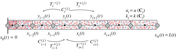
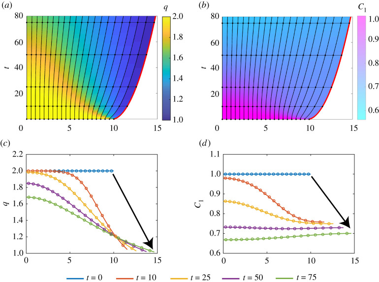
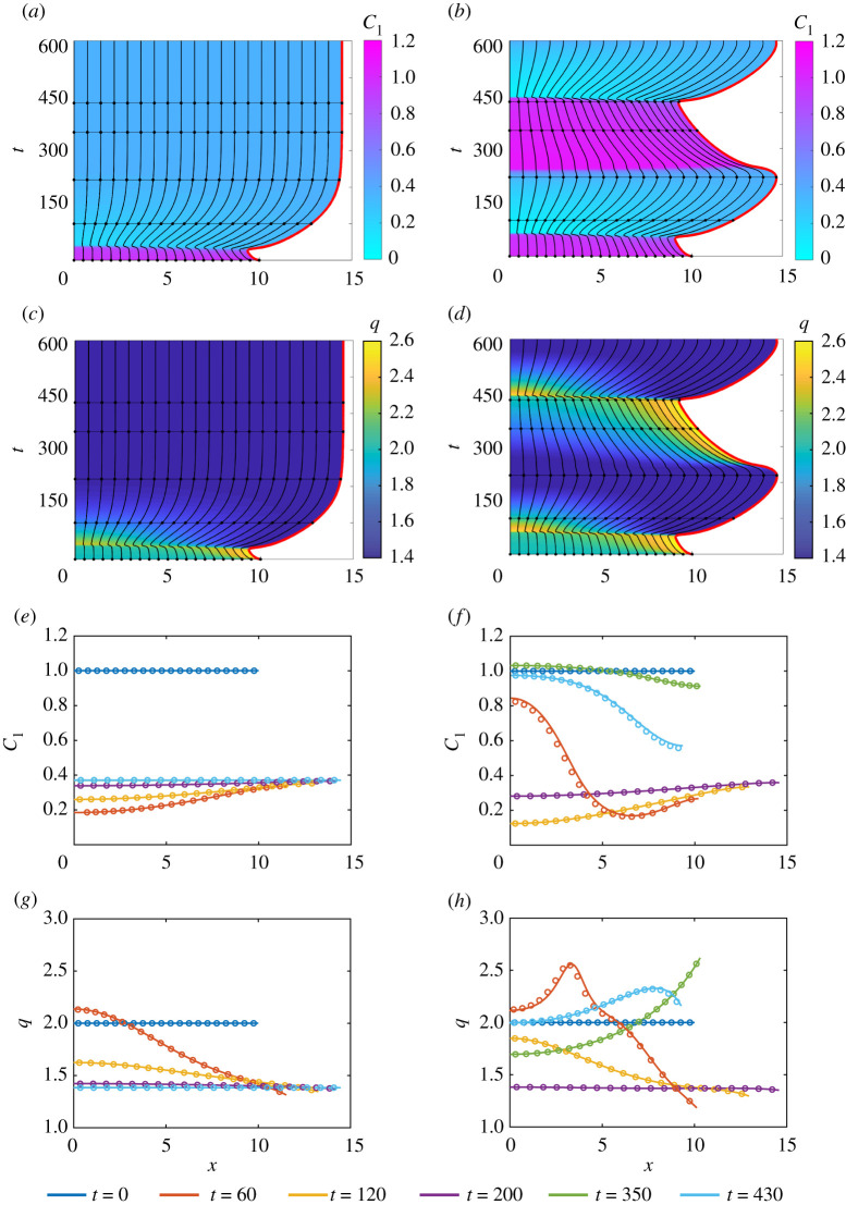
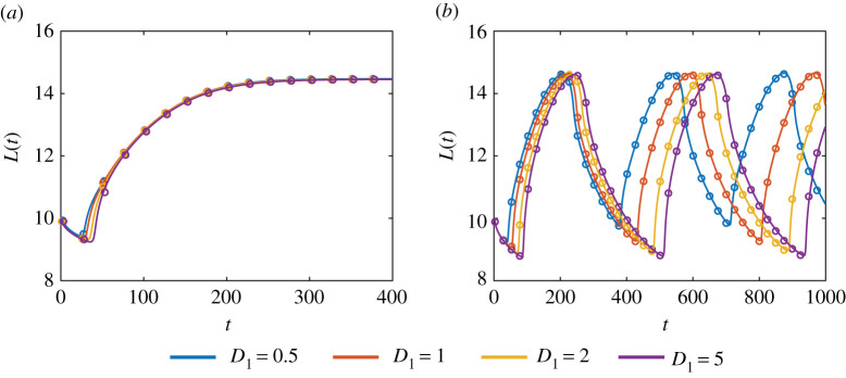
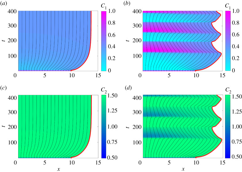
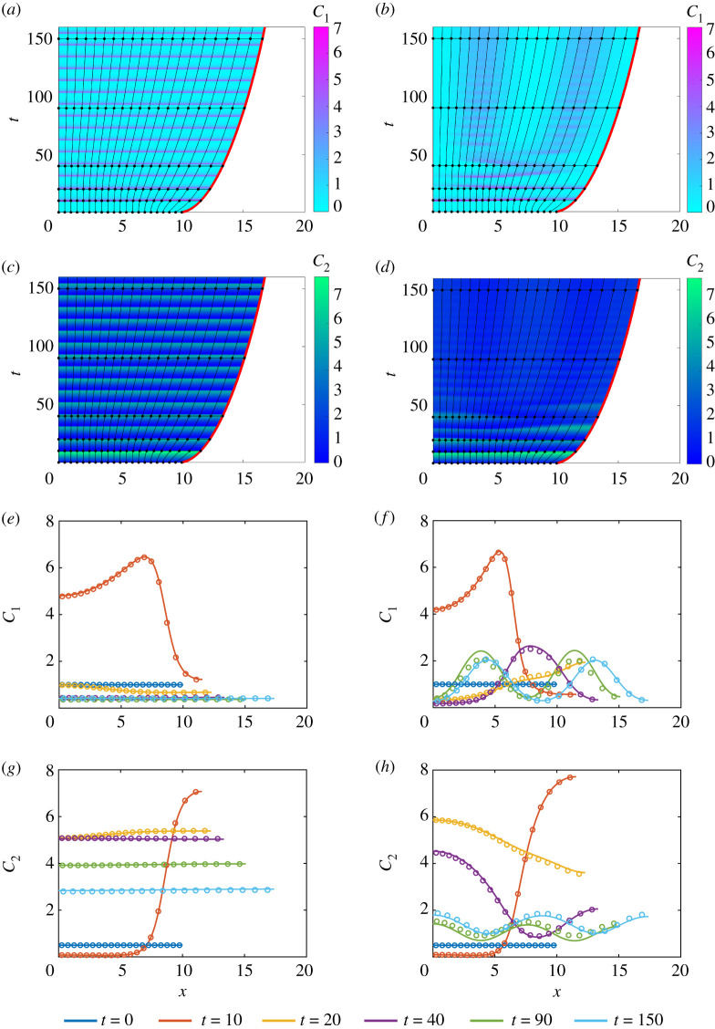
In this study, we couple intracellular signalling and cell-based mechanical properties to develop a novel free boundary mechanobiological model of epithelial tissue dynamics. Mechanobiological coupling is introduced at the cell level in a discrete modelling framework, and new reaction-diffusion equations are derived to describe tissue-level outcomes. The free boundary evolves as a result of the underlying biological mechanisms included in the discrete model. To demonstrate the accuracy of the continuum model, we compare numerical solutions of the discrete and continuum models for two different signalling pathways. First, we study the Rac-Rho pathway where cell- and tissue-level mechanics are directly related to intracellular signalling. Second, we study an activator-inhibitor system which gives rise to spatial and temporal patterning related to Turing patterns. In all cases, the continuum model and free boundary condition accurately reflect the cell-level processes included in the discrete model.

Keywords: cell-based model; continuum model; intracellular signalling; moving boundary problem; non-uniform growth; reaction–diffusion equations.

Figure 1.

Schematic of the discrete model where mechanical cell properties, a_i and k_i, are functions of the family of chemical signals, C_i(t). In this schematic, we consider two diffusing chemical species where the concentration in the ith cell is ${\mathbf{C}}_i(t)=\{C_i^{(1)}(t),C_i^{(2)}(t)\}$. The diffusive flux into cell i from cells i ± 1, and the diffusive flux out of cell i into cells i ± 1, is shown. Cell i, with boundaries at x_i−1(t) and x_i(t), is associated with a resident point, y_i(t), which determines the diffusive transport rates, $T_i^{\pm (j)}$. (Online version in colour.)

Figure 2.

Homogeneous tissue with N = 20 cells and one chemical species where $Z_1({\mathcal{C}}_1)=0$, and a = k = D₁ = η = 1. Characteristicdiagrams in (a,b) illustrate the position of cell boundaries where the free boundary is highlighted in red. The colour in (a,b) represents q(x, t) and ${\mathcal{C}}_1(x,t)$, respectively. In (a,b), the black horizontal lines indicate times at which q(x, t) and ${\mathcal{C}}_1(x,t)$ snapshots are shown in (c,d). In (c,d), the discrete and continuum solutions are compared as the dots and solid line, respectively, for t = 0, 10, 25, 50, 75 where the arrow represents the direction of time. (Online version in colour.)

Figure 3.

One-dimensional tissue dynamics where RhoA is coupled to mechanical cell tension. (a,c,e,g) correspond to β = 0.2 and (b,d,f ,h) relate to β = 0.3. Characteristic diagrams in (a–d) illustrate the evolution of cell boundaries where the free boundary is highlighted inred. The colour in (a,b) represents ${\mathcal{C}}_1(x,t)$ and q(x, t) in (c,d). The black horizontal lines indicate times at which ${\mathcal{C}}_1(x,t)$ and q(x, t) snapshots are shown in (e,f ) and (g,h), respectively. In (e–h), the discrete and continuum solutions are compared as the dots and solid line, respectively, for t = 0, 100, 220, 350, 430. In both systems, $a=l_0-\varphi {\mathcal{C}}_1^p/(G_{\mathrm{h}}^p+{\mathcal{C}}_1^p)$, $k=1+0.05{\mathcal{C}}_1$, D₁ = 1, η = 1 and ${\mathcal{C}}_1(0,t)=1$ for x ∈ [0, L(t)]. Parameters: b = 0.2, γ = 1.5, n = 4, p = 4, G_T = 2, l₀ = 1, ϕ = 0.65, G_h = 0.4, δ = 1. (Online version in colour.)

Figure 4.

The effect of diffusion on the dynamics of the free boundary for (a) a non-oscillatory system with β = 0.2 and (b) a oscillatory system with β = 0.3. The discrete solution is shown as the dots and the continuum solution as a solid line. Parameters are as in figure 3. (Online version in colour.)

Figure 5.

Characteristic diagrams for the interaction of RhoA and Rac1 where the free boundary is highlighted in red. Panels (a,c) correspond to a non-oscillatory system, where $\hat{\beta }=1$ and (b,d)relate to an oscillatory system where $\hat{\beta }=2.5$. The colour in (a,b) denotes the concentration of RhoA and the concentration of Rac1 in (c,d). In both systems, $a=l_0-\varphi {\mathcal{C}}_1^p/(G_{\mathrm{h}}^p+{\mathcal{C}}_1^p)$, $k=1+0.1{\mathcal{C}}_2$, D₁ = D₂ = 1 and η = 1. The initial conditions are ${\mathcal{C}}_1(0,t)=1$ and ${\mathcal{C}}_2(0,t)=0.5$ for x ∈ [0, L(t)]. Parameters: b₁ = b₂ = 1, δ₁ = δ₂ = 1, n = 3, p = 4, $G_{1_{\mathrm{T}}}=2$, $G_{2_{\mathrm{T}}}=3$, l₀ = 1, ϕ = 0.65, G_h = 0.4. Discrete and continuum solutions are compared in the electronic supplementary material, S5. (Online version in colour.)

Figure 6.

Activator–inhibitor patterns in a homogeneous tissue. In (a,c,e,g), D₁ = 2 and D₂ = 3 with d < d_c. In (b,d,f ,h), D₁ = 0.5 and D₂ = 5 with d > d_c. (a)–(d) shows the cellboundaries where the free boundary is highlighted in red. The colour in (a,b) represents ${\mathcal{C}}_1(x,t)$ and ${\mathcal{C}}_2(x,t)$ in (c,d). The black horizontal lines indicate times at which ${\mathcal{C}}_1(x,t)$ and ${\mathcal{C}}_2(x,t)$ snapshots are shown in (e,f ) and (g,h), respectively. In (e–h), the discrete (dots) and continuum (solid line) solutions are compared at t = 0, 10, 20, 40, 90, 150. In both systems, ${\mathcal{C}}_1(x,0)=1$ and ${\mathcal{C}}_2(x,0)=0.5$ for x ∈ [0, L(t)] and a = k = η = 1. Parameters: n₁ = 0.1, n₂ = 1, n₃ = 0.5, n₄ = 1 and d_c = 4.9842. (Online version in colour.)

Figure 7.

The evolution of spatial–temporal patterns in a homogeneous tissue with Schnakenberg dynamics, where d > d_c and k = 0.5. Characteristic diagrams in (a,b) illustrate the evolution of cell boundaries where the free boundary is highlighted in red. The colour in (a) represents ${\mathcal{C}}_1(x,t)$ and ${\mathcal{C}}_2(x,t)$in (b). The black horizontal lines indicate times at which ${\mathcal{C}}_1(x,t)$ and ${\mathcal{C}}_2(x,t)$ snapshots are shown in (c) and (d), respectively. In (c,d), the discrete and continuum solutions are compared as the dots and solid line, respectively, for t = 0, 10, 20, 40, 90, 200. The initial conditions are ${\mathcal{C}}_1(x,0)=1$ and ${\mathcal{C}}_2(x,0)=0.5$ for x ∈ [0, L(t)], with a = η = 1, D₁ = 0.5 and D₂ = 5. Parameters: n₁ = 0.1, n₂ = 1, n₃ = 0.5, n₄ = 1 and d_c = 4.9842. (Online version in colour.)