Frontiers in Multiscale Modeling of Photoreceptor Proteins

Abstract

This perspective article highlights the challenges in the theoretical description of photoreceptor proteins using multiscale modeling, as discussed at the CECAM workshop in Tel Aviv, Israel. The participants have identified grand challenges and discussed the development of new tools to address them. Recent progress in understanding representative proteins such as green fluorescent protein, photoactive yellow protein, phytochrome, and rhodopsin is presented, along with methodological developments.

Fig. 1.

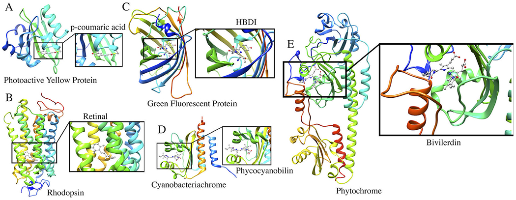
Photoreceptor proteins discussed in this perspective article. (A) Photoactive Yellow Protein with p-coumaric acid as a chromophore; (B) Rhodopsin with a retinal chromophore; (C) Green Fluorescent Protein with a HBDI chromophore; (D) Cyanobacteriochrome with phycocyanobilin as a chromophore; (E) Phytochrome with a Biliverdin chromophore.

Fig. 2.

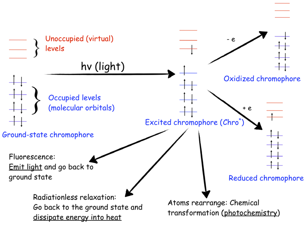
Excited-state processes in photoreceptor proteins. The photocycle of a chromophore, an acting core of a photoreceptor, involves various competing processes: fluorescence, radiationless relaxation, intersystem crossing (not shown), excited-state chemical transformations, and electron transfer. Reproduced with permission from Ref. (19).

Fig. 3.

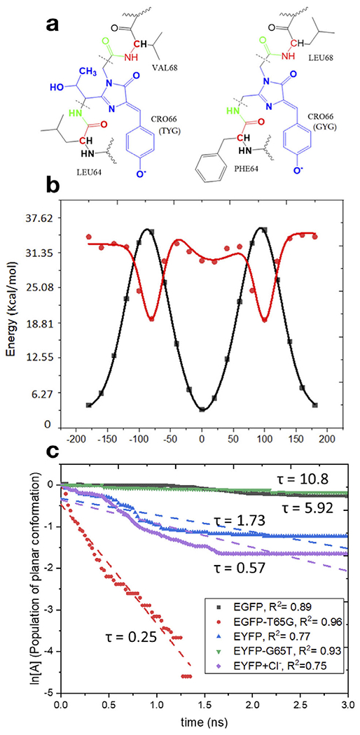
Top: Structures of the model proteins with the TYG (EGFP, YFP-G65T) (left) and GYG (YFP, EGFP-T65G) (right) chromophores and the definition of the QM/MM partitioning (the QM part is shown in blue and the MM part in black). The key difference between the TYG and GYG chromophores is the -C(OH)CH₃ tail in the latter. Bottom left: Potential energy along torsional angle φ (phenolate flip) in the ground and excited states. Bottom right: First-order kinetics of the chromophore’s twisting in the excited state in four model proteins. Reproduced with permission from Ref. (22).

Fig. 4.

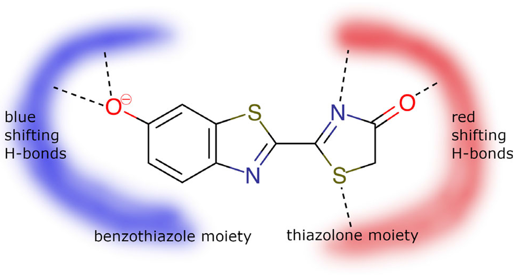
Oxyluciferin and the hydrogen-bonding networks responsible for blue- or red-shifted emission.

Fig. 5.

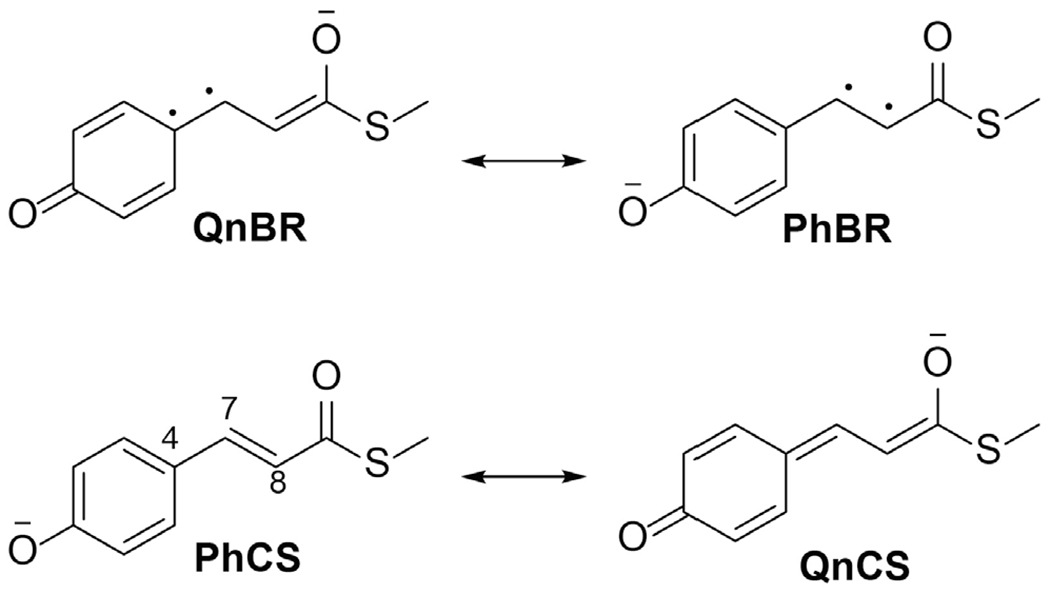
Resonance structures explaining the interdependent properties of the anionic pCT- chromophore of PYP derived in Ref. (53). C4-C7 and C7=C8 are the central single bond (SB) and double bond (DB), respectively.

Fig. 6.

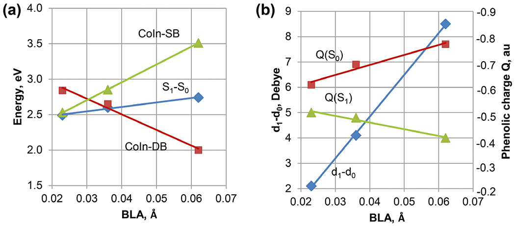
The linear correlation plots summarize the XMCQDPT2/cc-pVDZ results for the pCT- chromophore interacting with water molecules (53). Panels a and b show correlations for the energies and charge transfer, respectively. The bond length alternation (BLA) value corresponds to the difference in the length of the C4-C7 and C7=C8 bonds at the geometries fully optimized in the S₀ state.

Fig. 7.

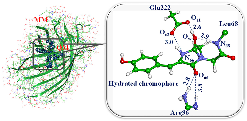
Left: a model system for simulations of the recovery reaction of the fluorescent state in Dreiklang. Right: a part of the system selected for QM/MM calculations of the reaction energy profile.

Fig. 8.

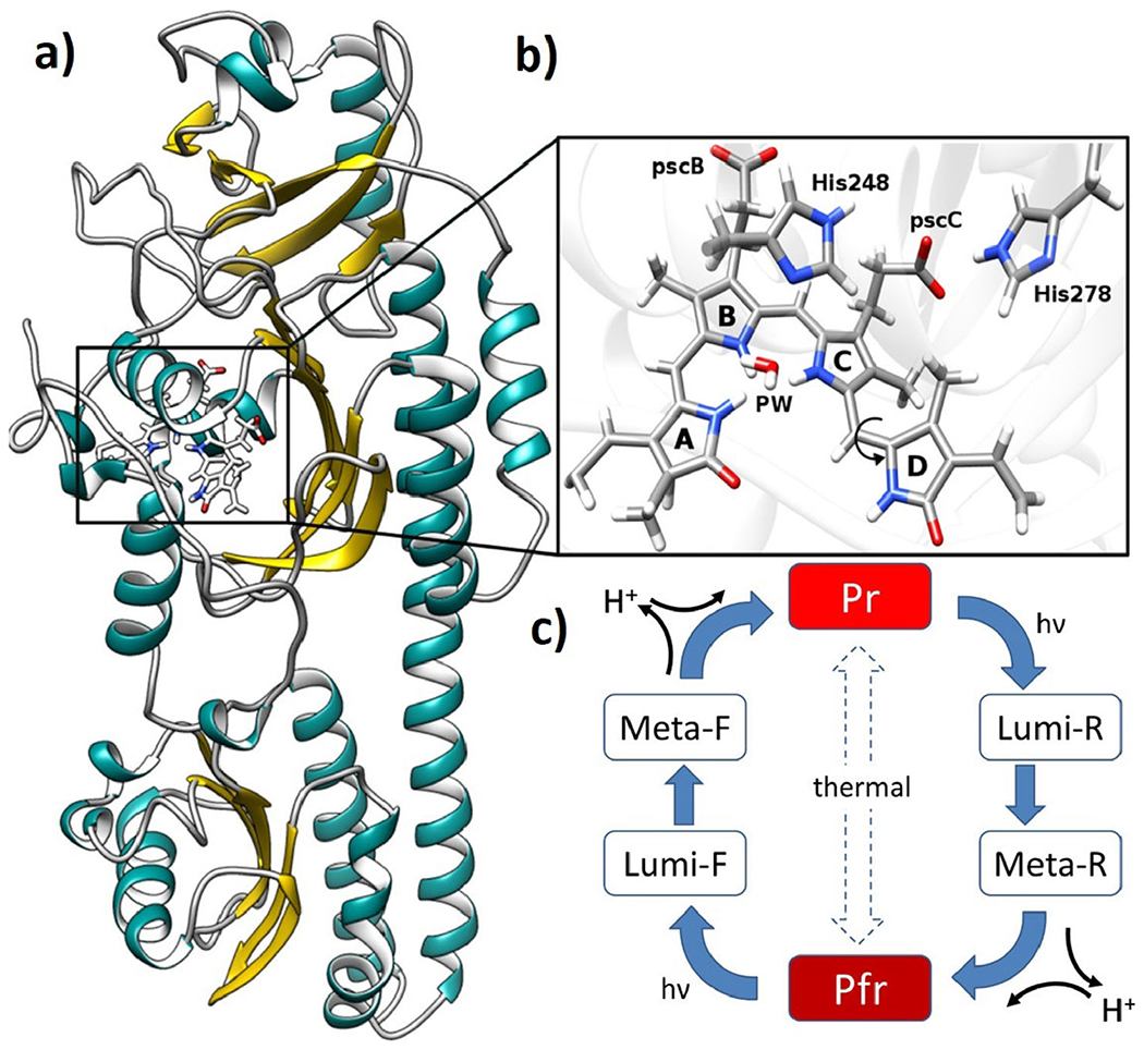
a) crystal structure of Agp2 phytochrome in Pfr state, b) BV chromophore, pyrrole water (PW) and histidines located in the chromophore binding pocket. c) generic phytochrome photocycle with the red light-absorbing parent state (Pr) and far-red light-absorbing parent state (Pfr).

Fig. 9.

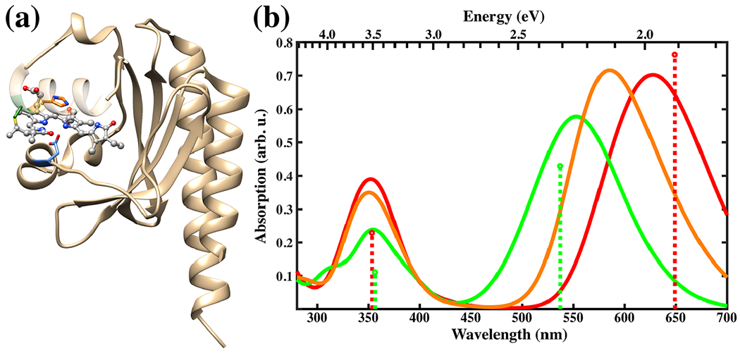
Left: Slr1393g3 protein structure in the Pr form. The PCB chromophore is shown in gray in the balls and sticks representation and the colors of selected sidechains are: CYS-528 in green, HIS-529 in orange and ASP-498 in blue. Right: Absorption spectra for the Pr (red), Pg (green) and Ph (orange) forms calculated with sTD-DFT based on CAM-B3LYP ground state calculations with a QM region consisting of PCB and the sidechains shown on the left. The spectra are based on 100 snapshots from a DFTB2+D/AMBER trajectory taken every 10 ps. The sticks represent the positions and relative absorption maxima for the Pr and Pg forms extracted from measured spectra (89).

Fig. 10.

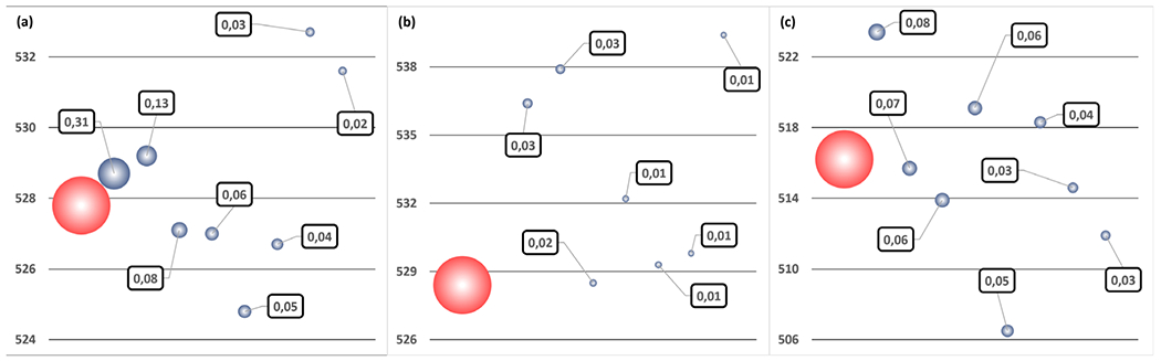
pH 3.5 (a), 5.5 (b), 7.5 (c) maximum absorption wavelength (in red) and the 8 most populated protonation microstate individual contributions (in gray). Wavelengths are given in nm. Bubble surfaces are proportional to microstate weights (squared labels), relatively to the complete ensemble.

Fig. 11.

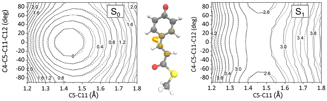
Reliability of interpolated PES: contour maps of the interpolated S₀ and S₁ state surfaces (solid lines) of the PYP chromophore in comparison with the reference quantum chemical data (dashed lines). Energy values are denoted in eV units. The contours were drawn by varying a torsional angle and its coupled bond length around the S₀-optimized geometry as denoted with the molecular structure. The interpolation data points were sampled in an iterative manner by adopting excited-state molecular dynamics simulations. The size of the interpolation data set was 2100.

Fig. 12.

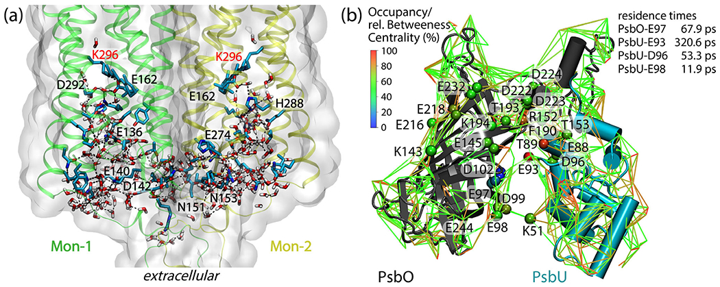
Dynamic hydrogen-bond networks in complex bio-systems. (a)t Extensive protein–water hydrogen-bond network in the extracellular halves of monomers Mon-1 and Mon-2 of the C1C2 dimer. The protein is shown as ribbons and molecular surfaces, and selected protein groups are shown as bonds with carbon atoms colored cyan, nitrogen—blue, and oxygen—red. For clarity, we label only protein groups part of a shortest-distance path that connects the two retinal Schiff bases. The molecular graphics and the path analyses are based on ref. (108). (b): Protein–water hydrogen-bond network at the surface of the soluble PsbO and PsbU subunits of photosystem II. Lines inter-connect charged and polar sidechains via hydrogen-bonded water bridges; for clarity, we display water bridges that are present during at least 50% of a simulation of the PsbO-PsbU complex in aqueous solution. Cα of amino acid residues are colored according to relative betweenness centrality values. Lines are color-coded, according to occupancy values. The image and the centrality computations are based on Ref. (109)

Fig. 13.

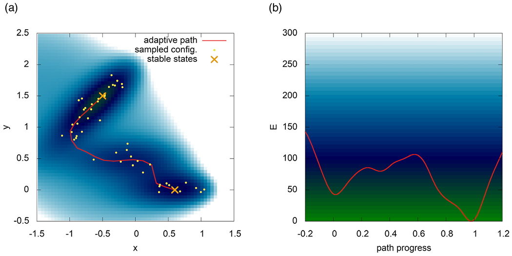
An adaptive path-CV captures the transition channel on the Müller–Brown (120) potential energy surface.

Fig. 14.

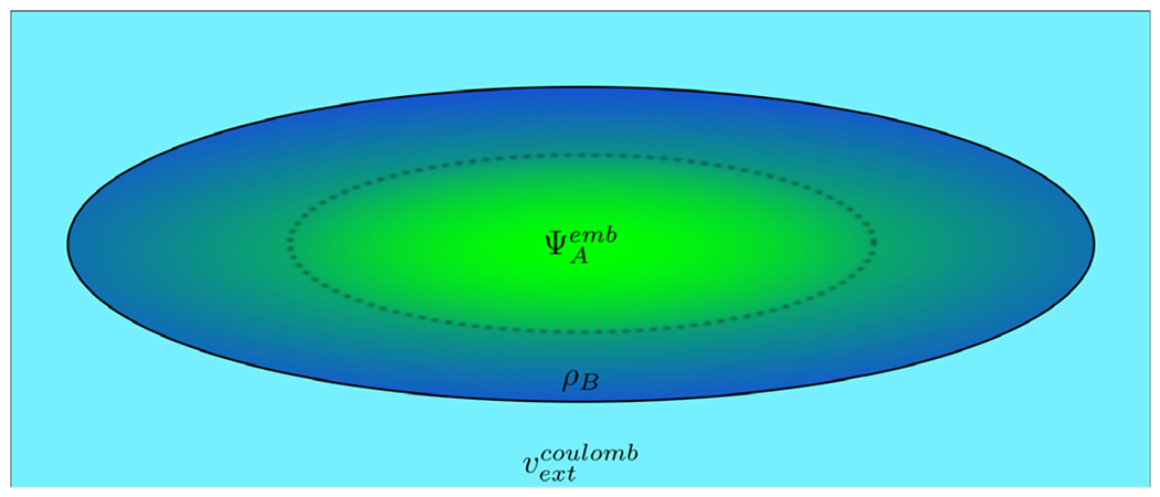
Scheme of the FDET model of a chromophore embedded in a protein. Different colors represent regions in 3D space which are described using different descriptors: embedded Ψ_A for the chromophore (green) and density ρ_B(r) for its nearest neighbors (dark blue). Note that these regions can overlap. If needed, the long range effects on the embedded wavefunction can be accounted for by means of a Coulombic potential v_ext^Coulomb.

Fig. 15.

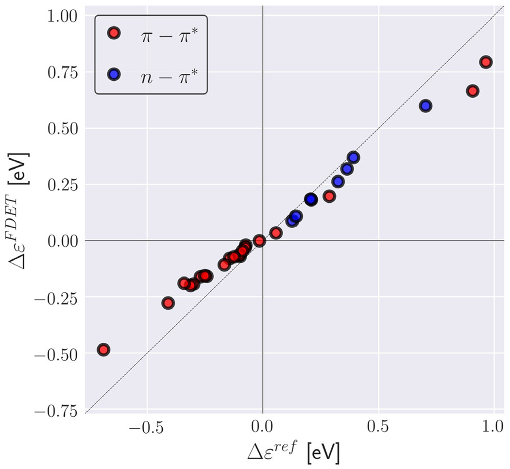
Environment-induced shifts of the lowest vertical excitation energy for organic chromophores in hydrogen-bonded environments (XH-27 dataset from Ref. (144)). Reference shifts (Δϵ^ref) are taken Ref. (144) (excitation energy shifts obtained from ADC(2) calculations for the whole clusters). FDET shifts (Δϵ^FDET) are obtained from embedded ADC (2) calculations as described in Ref. (144) except the reduction of the number of centers in the basis sets used for Ψ_A and ρ_B (monomer expansion is used here).

Fig. 16.

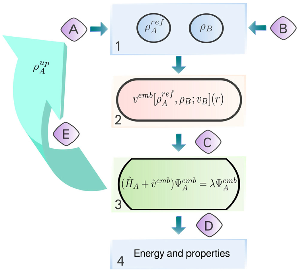
General workflow of a FDET-based simulation. The main steps, given in square boxes, can be performed using various standard quantum chemistry codes: 1—generation of ρ_A(r) and ρ_B(r) in real space, 2—generation of the embedding potential in real space, 3—obtaining embedded N_A-electron wavefunction (variational or not) from a user-chosen quantum chemistry method and code; 4—a posteriori evaluation of the FDET energy components which depend on the method used in step 3 and other properties. Interfacing is performed by subroutines indicated with capital letters: A—generation of initial N_A-electron density ρ_A ^ref(r); B—generation of ρ_B(r) (superposition of atomic or molecular densities, statistical ensemble averaging, pre-polarization, freeze-and-thaw optimization, etc.); C—generation of the embedding potential in atomic basis set representation (it can include an additional electrostatic field component as shown in Fig. 14); D—extracting quantities obtained in step 2 for step 3; E—iterative update of the embedding potential for verification of the linearization approximation (optional).

Fig. 17.

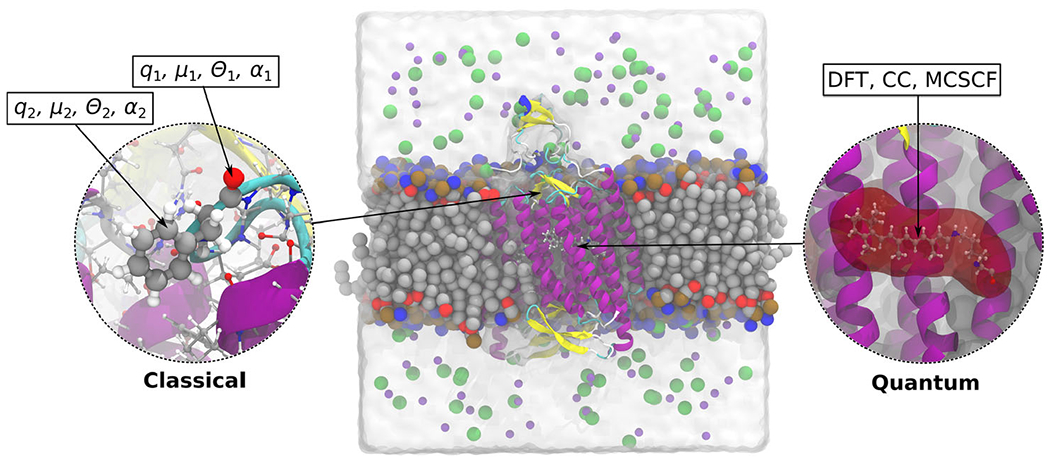
Illustration of the PE model applied on the membrane-embedded C1C2 channelrhodopsin. The active part, a protonated retinylidene Schiff base, is modeled using DFT/WFT, while the effect from the chromophores environment is modeled classically using atom-centered multipoles and polarizabilities.

Fig. 18.

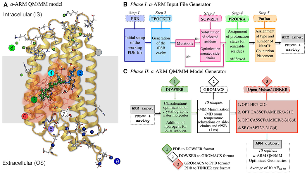
Structure of the a-ARM rhodopsin model building protocol. (A) General scheme of a QM/MM model generated by a-ARM for a Type I rhodopsin. This is composed of: (1) environment subsystem (gold cartoon), (2) retinal chromophore (green tubes), (3) Lys side-chain covalently linked to the retinal chromophore (blue tubes), (4) main counter-ion MC (cyan tubes), (5) residues with non-standard protonation states, (6) residues of the chromophore cavity subsystem (red tubes), (7) water molecules, and external (8) Cl⁻ (green balls) and (9) Na⁺ (blue balls) counterions. The external extracellular (OS) and intracellular (IS) charged residues are shown in frame representation. (right) General workflow of the a-ARM rhodopsin model building protocol for the generation of QM/MM models of wild-type and mutant rhodopsins. The a-ARM protocol comprises two phases: (B) input file preparation phase and (C) QM/MM model generator phase.

Fig. 19.

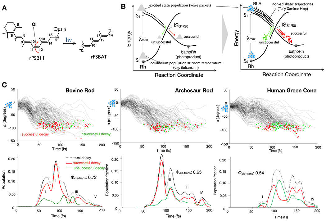
Rhodopsin population dynamics. (A) 11-cis retinal chromophore (rPSB11 for Type II rhodopsins such as Rh) photoisomerization and isomerizing torsional angle α (C10-C11-C12-C13 dihedral angle). (B) Schematic representation of the light-triggered ultrafast population dynamics of Rh. IS_S1/S0 (48,162) stands for intersection space between the ground state (S₀) and the first singlet excited state (S₁) representing collectively the points of decay (hop) to the ground state (S₀). The reaction coordinate is complex but it is mainly driven by the α angle. The diagram on the right represents a non-adiabatic trajectory calculation where the initial vibrational wave-packet (or population) is represented by a collection of initial conditions (structures and velocities) indicated by light-blue circles and one trajectory is propagated from each initial condition point. (C) The time progression of α along a set of 200 non-adiabatic trajectories simulating the S₁ population dynamics of bovine rhodopsin at room temperature is given in the top-left panel. The bottom-left panel gives the statistic of successful and unsuccessful hops as a function of time. The computed quantum efficiency value is also given. The circles represent decay from S₁ to S₀ with a red circle representing successful decays leading to the photoproduct while green circles lead to the reactant. Center. Same results for a model reconstructed from an amino acid sequence obtained via phylogenetic analysis and ancestral sequence reconstruction techniques (163,164). Right. Same data for the opsin from a human green cone receptor cell.

Fig. 20.

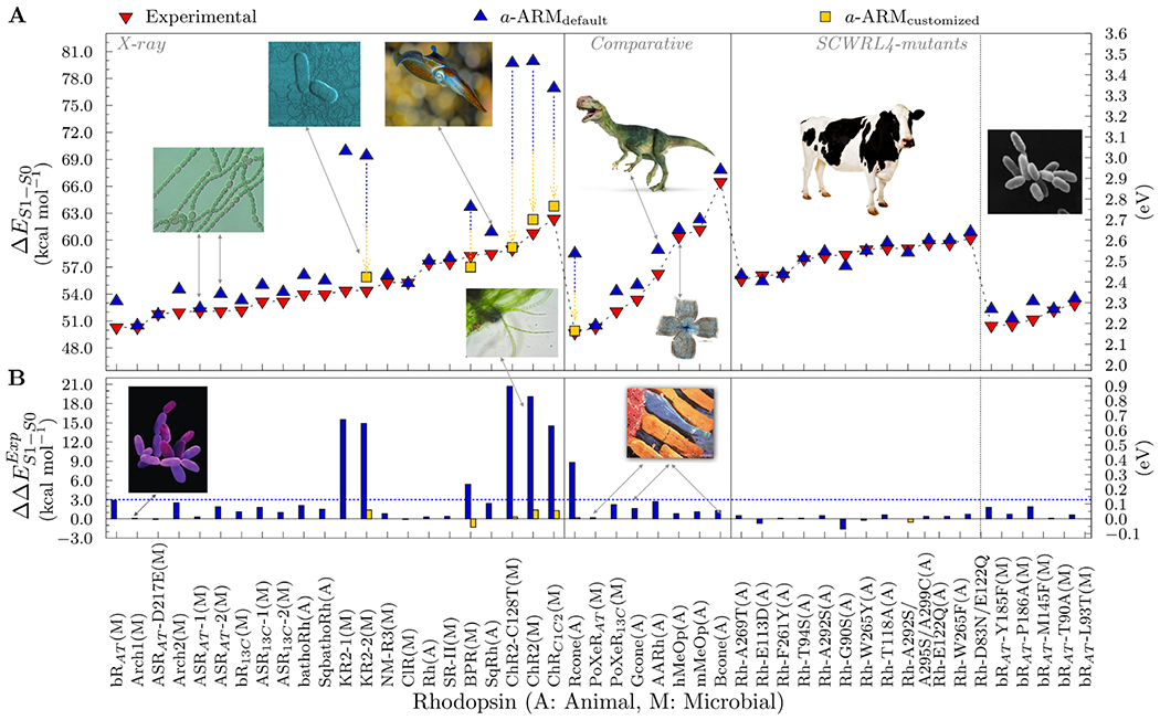
Benchmarking of a-ARM. (A) Computed excitation energies ΔE_S1-S0 in both kcal mol⁻¹ (left axis) and eV (right axis) for various rhodopsins. The employed protein structures where obtained from X-ray crystallography (left panel) or through comparative modeling (center panel). Two sets of variants for bovine rhodopsin (Rh) and bacteriorhodopsin (bR) are also reported (right panel). The computed data were obtained using the a-ARM_default (blue up-turned triangles) and a-ARM_customized (gold squares). Experimental data, as energy difference corresponding to the wavelength of the absorption maxima, are also reported (red down-turned triangles). (B) Differences between computed and experimental excitation energies ΔΔE ^Exp_S1-S0 in both kcal mol⁻¹ (left axis) and eV (right axis).

Fig. 21.

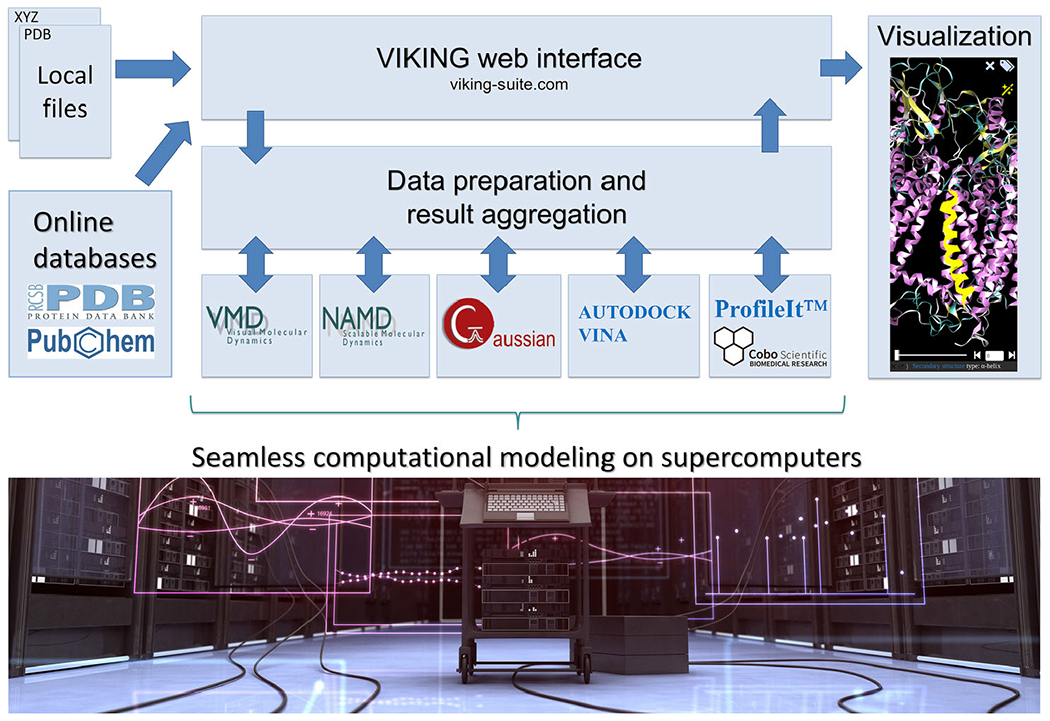
Concept and workflow of VIKING. Computational tasks are configured in the web interface by supplying the input data (structures, potentials, input field values etc), from the local computer or an online database. The simulation is then performed on a supercomputer (Stampede2, Marconi and Abacus 2.0 are currently supported), the results are aggregated and represented visually in the web browser. Supercomputer photograph courtesy of iStockphoto LP. Copyright 2012.

References

-
- Van Der Horst MA and Hellingwerf KJ (2004) Photoreceptor proteins, “star actors of modern times”: A review of the functional dynamics in the structure of representative members of six different photoreceptor families. Acc. Chem. Res 37(1), 13–20. - PubMed
- Zimmer M (2002) Green fluorescent protein (GFP): applications, structure, and related photophysical behavior. Chem. Rev 102(3), 759–781. - PubMed
- Reis JM and Andrew Woolley G (2016) Photo control of protein function using photoactive yellow protein. In: Methods in Molecular Biology, Vol. 1408, pp. 79–92.Humana Press Inc. - PubMed
- Meech SR (2009) Excited state reactions in fluorescent proteins. Chem. Soc. Rev 38(10), 2922–2934. - PubMed
Publication types
MeSH terms
Substances
Grants and funding
LinkOut - more resources
Full Text Sources
Other Literature Sources