

FLIMJ: An open-source ImageJ toolkit for fluorescence lifetime image data analysis
- PMID: 33378370
- PMCID: PMC7773231
- DOI: 10.1371/journal.pone.0238327
FLIMJ: An open-source ImageJ toolkit for fluorescence lifetime image data analysis
Abstract
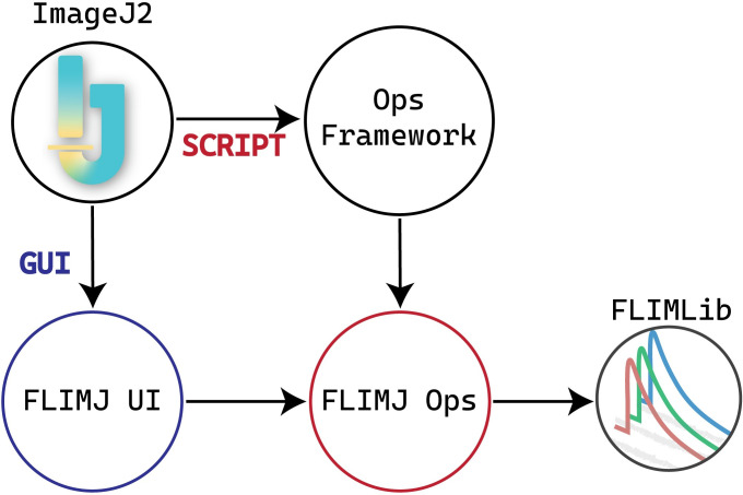
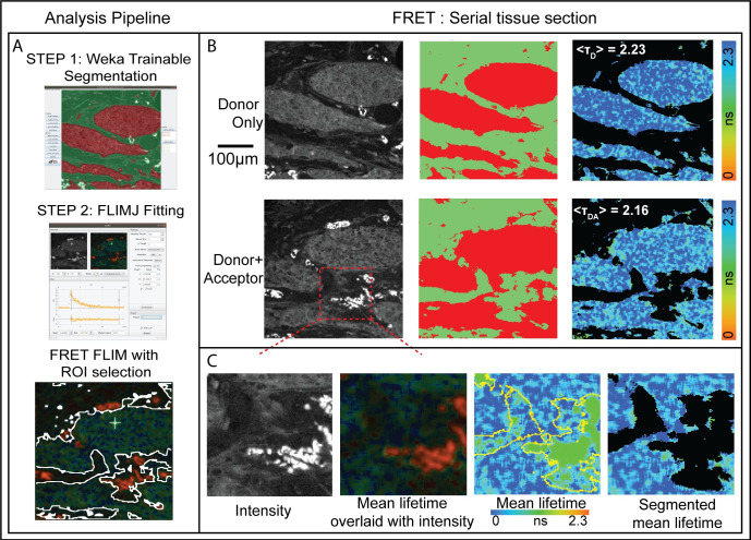
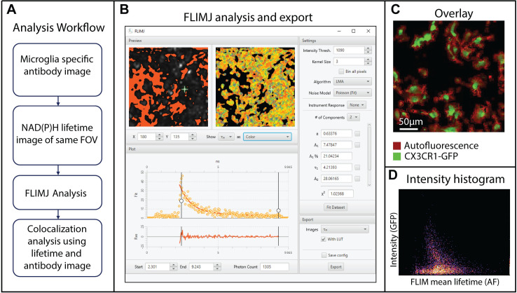
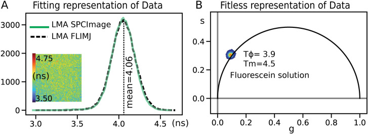
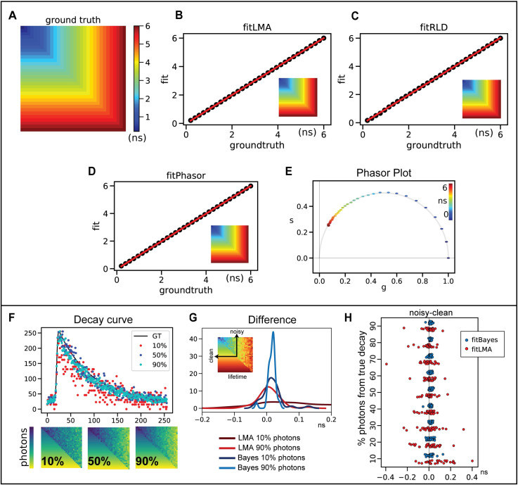
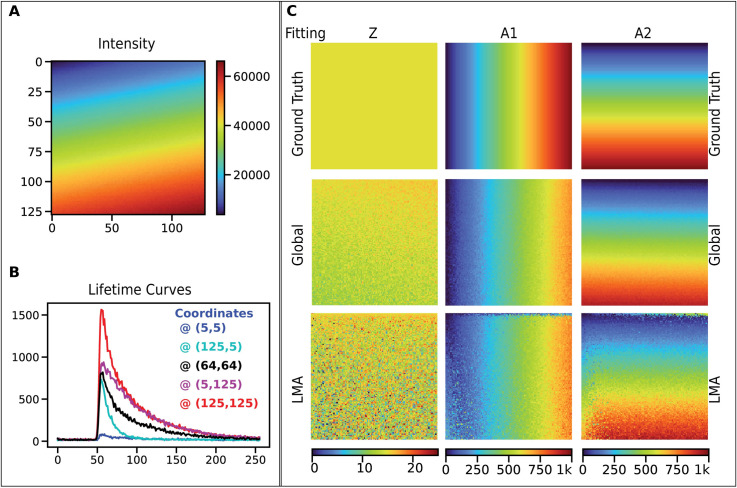
In the field of fluorescence microscopy, there is continued demand for dynamic technologies that can exploit the complete information from every pixel of an image. One imaging technique with proven ability for yielding additional information from fluorescence imaging is Fluorescence Lifetime Imaging Microscopy (FLIM). FLIM allows for the measurement of how long a fluorophore stays in an excited energy state, and this measurement is affected by changes in its chemical microenvironment, such as proximity to other fluorophores, pH, and hydrophobic regions. This ability to provide information about the microenvironment has made FLIM a powerful tool for cellular imaging studies ranging from metabolic measurement to measuring distances between proteins. The increased use of FLIM has necessitated the development of computational tools for integrating FLIM analysis with image and data processing. To address this need, we have created FLIMJ, an ImageJ plugin and toolkit that allows for easy use and development of extensible image analysis workflows with FLIM data. Built on the FLIMLib decay curve fitting library and the ImageJ Ops framework, FLIMJ offers FLIM fitting routines with seamless integration with many other ImageJ components, and the ability to be extended to create complex FLIM analysis workflows. Building on ImageJ Ops also enables FLIMJ's routines to be used with Jupyter notebooks and integrate naturally with science-friendly programming in, e.g., Python and Groovy. We show the extensibility of FLIMJ in two analysis scenarios: lifetime-based image segmentation and image colocalization. We also validate the fitting routines by comparing them against industry FLIM analysis standards.
Conflict of interest statement
The authors have declared that no competing interests exist.
Figures
Similar articles
-
New Extensibility and Scripting Tools in the ImageJ Ecosystem.Curr Protoc. 2021 Aug;1(8):e204. doi: 10.1002/cpz1.204. Curr Protoc. 2021. PMID: 34370407 Free PMC article.
-
Fluorescence lifetime imaging--techniques and applications.J Microsc. 2012 Aug;247(2):119-36. doi: 10.1111/j.1365-2818.2012.03618.x. Epub 2012 May 24. J Microsc. 2012. PMID: 22621335 Review.
-
phi2FLIM: a technique for alias-free frequency domain fluorescence lifetime imaging.Opt Express. 2009 Dec 7;17(25):23181-203. doi: 10.1364/OE.17.023181. Opt Express. 2009. PMID: 20052246
-
Imaging Vacuolar Anthocyanins with Fluorescence Lifetime Microscopy (FLIM).Methods Mol Biol. 2018;1789:131-141. doi: 10.1007/978-1-4939-7856-4_10. Methods Mol Biol. 2018. PMID: 29916076
-
[Fluorescence lifetime imaging microscopy (FLIM) in biological and medical research].Postepy Biochem. 2009;55(4):434-40. Postepy Biochem. 2009. PMID: 20201357 Review. Polish.
Cited by
-
New Extensibility and Scripting Tools in the ImageJ Ecosystem.Curr Protoc. 2021 Aug;1(8):e204. doi: 10.1002/cpz1.204. Curr Protoc. 2021. PMID: 34370407 Free PMC article.
-
Hyperdimensional Imaging Contrast Using an Optical Fiber.Sensors (Basel). 2021 Feb 9;21(4):1201. doi: 10.3390/s21041201. Sensors (Basel). 2021. PMID: 33572130 Free PMC article.
-
The ImageJ ecosystem: Open-source software for image visualization, processing, and analysis.Protein Sci. 2021 Jan;30(1):234-249. doi: 10.1002/pro.3993. Epub 2020 Nov 20. Protein Sci. 2021. PMID: 33166005 Free PMC article.
-
SciJava Ops: an improved algorithms framework for Fiji and beyond.Front Bioinform. 2024 Sep 27;4:1435733. doi: 10.3389/fbinf.2024.1435733. eCollection 2024. Front Bioinform. 2024. PMID: 39399098 Free PMC article.
-
The BrightEyes-TTM as an open-source time-tagging module for democratising single-photon microscopy.Nat Commun. 2022 Dec 1;13(1):7406. doi: 10.1038/s41467-022-35064-0. Nat Commun. 2022. PMID: 36456575 Free PMC article.
References
-
- Rueden CT, Conklin MW, Provenzano PP, Keely PJ, Eliceiri KW. Nonlinear optical microscopy and computational analysis of intrinsic signatures in breast cancer. 2009 Annual International Conference of the IEEE Engineering in Medicine and Biology Society. 2009. pp. 4077–4080. 10.1109/IEMBS.2009.5334523 - DOI - PMC - PubMed
Publication types
MeSH terms
Grants and funding
LinkOut - more resources
Full Text Sources
Molecular Biology Databases
