Hybrid methods for combined experimental and computational determination of protein structure

Abstract

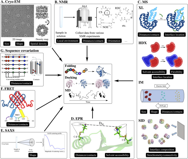
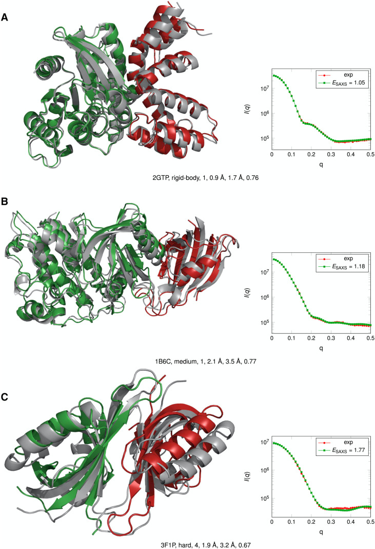
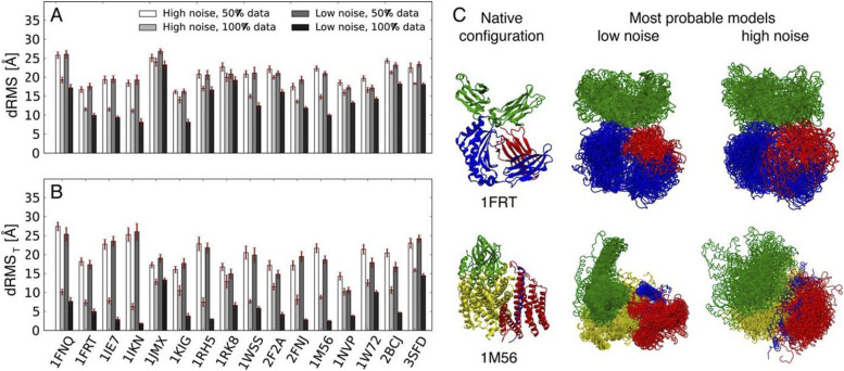
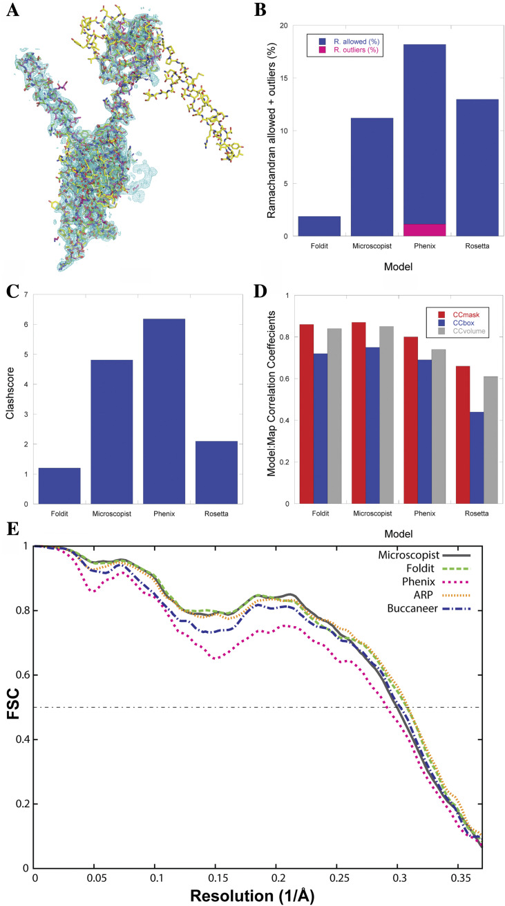
Knowledge of protein structure is paramount to the understanding of biological function, developing new therapeutics, and making detailed mechanistic hypotheses. Therefore, methods to accurately elucidate three-dimensional structures of proteins are in high demand. While there are a few experimental techniques that can routinely provide high-resolution structures, such as x-ray crystallography, nuclear magnetic resonance (NMR), and cryo-EM, which have been developed to determine the structures of proteins, these techniques each have shortcomings and thus cannot be used in all cases. However, additionally, a large number of experimental techniques that provide some structural information, but not enough to assign atomic positions with high certainty have been developed. These methods offer sparse experimental data, which can also be noisy and inaccurate in some instances. In cases where it is not possible to determine the structure of a protein experimentally, computational structure prediction methods can be used as an alternative. Although computational methods can be performed without any experimental data in a large number of studies, inclusion of sparse experimental data into these prediction methods has yielded significant improvement. In this Perspective, we cover many of the successes of integrative modeling, computational modeling with experimental data, specifically for protein folding, protein-protein docking, and molecular dynamics simulations. We describe methods that incorporate sparse data from cryo-EM, NMR, mass spectrometry, electron paramagnetic resonance, small-angle x-ray scattering, Förster resonance energy transfer, and genetic sequence covariation. Finally, we highlight some of the major challenges in the field as well as possible future directions.

FIG. 1.

Representations of each featured experimental method used for computational modeling. In this Perspective, we discuss how each method has been used for computational modeling in the form of de novo folding from the sequence (tertiary structure prediction), protein–protein docking (quaternary structure prediction), and molecular dynamics (physics-based protein dynamics simulation), as shown in the center panel. In the outer panels, each experimental method is tagged based on the type of structural information provided by its data. The categories are size, shape, solvent accessibility, interface location/composition, distances/contacts, spatial density, orientation, local environment, flexibility, and stoichiometry/connectivity. (a) Cryo-EM 2D projection image of the GroEL complex, a homo 14-mer with D7 symmetry, in vitreous ice is shown on the left. Some examples of individual projections of the complex in different orientations are circled. On the right, the reconstructed 3D density map of the complex at 3.5 Å resolution (EMDB: 8750) is shown in two orientations. Cryo-EM density maps provide information on size, shape, and spatial density. (b) Representations of the most common forms of NMR data used for integrative structural modeling. Chemical shifts (CSs) provide information on local environments, nuclear Overhauser effect (NOE) provides distance between atom pairs, and residual dipolar coupling (RDC) provides information on inter-nuclei vector orientations. (c) Representations of various mass spectrometry (MS) methods that encode structural information into protein/peptide mass. Chemical cross-linking (XL) provides distances between residues that are cross-linked by fixed-length reagents and can provide the interface location when performed on a complex. In hydrogen–deuterium exchange (HDX), the exchange rates (from H to D of backbone amide hydrogens) provide information on solvent exposure and flexibility. By performing HDX on monomers and the complex (ΔHDX) and analyzing the difference, the interface location can also be determined. Ion mobility (IM) provides information on size and shape by separation, where larger proteins travel (left to right in this figure) through the bath gas with a lower velocity. This velocity can be used to calculate an averaged 2D collision cross section. If enough measurements are made on a protein complex and monomers, distances between subunits can also be approximated. Surface-induced dissociation (SID), which is exclusively used on complexes, can provide information on overall complex stoichiometry and subunit connectivity by breaking apart non-covalent interface interactions. Additionally, depending on the amount of energy required to break certain interfaces, a metric that depends on interface composition can also be measured. (d) Electron paramagnetic resonance (EPR) provides distances between paramagnetic spin labels, commonly nitroxide (spin-labeled residues shown as sticks). Because of the movement of spin labels, the location can be modeled using a cone as shown in this figure. The solvent accessibility of the paramagnetic labels can also be measured. (e) Small-angle x-ray scattering (SAXS) provides information on shape in the form of a scattering profile (scattering intensity as a function of spatial frequency), which can be approximated from the 3D structure. (f) Förster resonance energy transfer (FRET) can be measured by attaching a donor and acceptor fluorophore to the protein (either in vivo or in vitro) such as cyan fluorescent protein (CFP, shown in cyan) and yellow fluorescent protein (YFP, shown in yellow). The measured FRET efficiency (E_FRET) is dependent on the distance between the probes. (g) By performing a multiple sequence alignment with a large number of evolutionarily related sequences and identifying coevolving residue pairs, distance restraints or contacts can be determined.

FIG. 2.

Comparison of the utility of different types of information (green: contacts; orange: interface; and blue: EM density) for protein–protein docking. Docking results for a benchmark set of 162 complexes were evaluated based on the success rate (percentages of cases with a good model in the top N = 1, 10, 20, 100, or all), Fnat (fraction of native contacts), L-RMSD (ligand RMSD), and I-RMSD (interface RMSD). For all metrics, information on EM density was the most beneficial for integrative modeling. Reprinted with permission from de Vries et al., Biophys. J. 110(4), 785–797 (2016). Copyright 2016 Cell Press.

FIG. 3.

Improvement in fit to the density map using MDFF for acethyl-CaA synthase. Target structures and simulated density maps are shown in gray, and the initial and fitted structures are shown in green (top) and colored by backbone RMSD (Å) per residue (bottom). After MDFF, there was a significant improvement both in density map fit and RMSD. Reprinted with permission from Trabuco et al., Structure 16(5), 673–683 (2008). Copyright 2008 Cell Press.

FIG. 4.

NMR restraints improved native-like sampling in BCL. Each point signifies one protein. Points are colored based on size (green: <150 residues; yellow: ≥150 and <250 residues; orange: ≥250 and <400 residues; and red: ≥400 residues) and shaped based on type (circle: soluble and square: membrane). (a) The mean RMSD100 with error bars of ±1 SD of the top 10 models with (y-axis) and without (x-axis) NMR restraints. (b) The RMSD100 of the top model with and without NMR restraints. Reprinted with permission from Weiner et al., Proteins 82(4), 587–595 (2014). Copyright 2014 John Wiley and Sons.

FIG. 5.

MELDxMD was the highest ranked group in NMR data-assisted CASP13 (2018). (a) MELDxMD (431) had the highest Z-score in the category. (b) Predicted structures for CASP targets are shown with reference to the native structures. Five of these predicted structures were best in CASP. Reprinted with permission from Robertson et al., Proteins 87(12), 1333–1340 (2019). Copyright 2019 John Wiley and Sons.

FIG. 6.

The inclusion of HRF data improved structure prediction for myoglobin. Top shows score vs RMSD plots and quality of funneling metric, P_near, for 20 000 ab initio models (top scoring model for each shown with a star). Bottom shows a comparison of top scoring model (cyan) to the crystal structure (gray). Results are shown for when no HRF data were included (left), when hrf_dynamics score was included (middle), and when hrf_dynamics score was included with further sampling using Rosetta movers for the top 20 models (right). Figure credit: Sarah Biehn.

FIG. 7.

Comparison of predicted subcomplexes with (left, blue) and without (right, red) the inclusion of SID data into protein–protein docking. The native structures are shown for reference (green). RMSD (Å) to the mobile chain is shown. RMSD improved by >18 Å when SID data were included for these cases. Reprinted with permission from Seffernick et al., ACS Cent. Sci. 5(8), 1330–1341 (2019). Copyright 2019 American Chemical Society (ACS). Further permissions related to the material excerpted should be directed to the ACS.

FIG. 8.

Comparison of sampling for Bax and ExoU de novo folding using DEER data to predict structures. RosettaDEER showed improvement in sampling over the previous cone method and when no EPR restraints were included. Reprinted with permission from Del Alamo et al., Biophys. J. 118(2), 366–375 (2020). Copyright 2020 Cell Press.

FIG. 9.

Docked structures generated using ATTRACT-SAXS for an easy [(a) 2GTP], medium [(b) 1B6C], and hard [(c) 3F1P] case. Docked models are shown in green and red, and the crystal structure is shown in gray along with the cluster rank, IRMSD, LRMSD, and fnat. For comparison, the simulated SAXS profiles are also shown along with the experimental curves. Reprinted with permission from Schindler et al., Structure 24(8), 1387–1397 (2016). Copyright 2016 Cell Press.

FIG. 10.

Benchmark of FRET-based modeling in the integrative modeling platform. The accuracy (average C-α RMSD between crystal structure and 20 most probable models) of the modeled structures as a function of noise and data sparseness is shown for (a) all residues and (b) N- and C-terminal residues. Because the FRET tags were placed on the termini, the accuracy of the models was significantly better [(b) vs (a)]. (c) The ensemble of the most probably models compared to the native for 1FRT and 1M56. Reprinted with permission from Bonomi et al., Mol. Cell Proteomics 13(11), 2812–2823 (2014). Copyright 2014 American Society for Biochemistry and Molecular Biology (United States).

FIG. 11.

Performance of AlphaFold (A7D) in CASP13 (2018). Number of free modeling domains predicted for a given TM-score threshold for AlphaFold (blue) and other groups (red). Reprinted with permission from Senior et al., Proteins 87(12), 1141–1148 (2019). Copyright 2019 John Wiley and Sons.

FIG. 12.

(a) Comparison of models for Afp7. The Foldit structure is rendered in green, the microscopist structure in gray, the Phenix model in magenta, and the Rosetta model in yellow. The electron potential map is contoured at 2σ. (b) Comparison of the Ramachandran outlier and allowed backbone conformations. (c) Comparison of Molprobity Clashscore—in both cases, lower is better. (d) Comparison of three different map-to-model correlation coefficients in which higher values are better. (e) Map-to-model FSC curves for Microscopist (gray), Foldit (green), Phenix (pink), ARP w/ARP (orange), and Buccaneer (blue) models. Reprinted with permission from Khatib et al., PLoS Biol. 17(11), e3000472 (2019). Copyright 2019.

References

1. Leelananda S. P. and Lindert S., “Computational methods in drug discovery,” Beilstein J. Org. Chem. 12, 2694–2718 (2016). 10.3762/bjoc.12.267 - DOI - PMC - PubMed
1. Nwanochie E. and Uversky V. N., “Structure determination by single-particle cryo-electron microscopy: Only the sky (and intrinsic disorder) is the limit,” Int. J. Mol. Sci. 20(17), 4186 (2019). 10.3390/ijms20174186 - DOI - PMC - PubMed
1. Würz J. M., Kazemi S., Schmidt E., Bagaria A., and Güntert P., “NMR-based automated protein structure determination,” Arch. Biochem. Biophys. 628, 24–32 (2017). 10.1016/j.abb.2017.02.011 - DOI - PubMed
1. Ilari A. and Savino C., “Protein structure determination by x-ray crystallography,” Methods Mol. Biol. 452, 63–87 (2008). 10.1007/978-1-60327-159-2_3 - DOI - PubMed
1. Overall Growth of Released Structures per Year, RCSB, 2020.