Using a GTR+Γ substitution model for dating sequence divergence when stationarity and time-reversibility assumptions are violated

Abstract

Motivation: As the number and diversity of species and genes grow in contemporary datasets, two common assumptions made in all molecular dating methods, namely the time-reversibility and stationarity of the substitution process, become untenable. No software tools for molecular dating allow researchers to relax these two assumptions in their data analyses. Frequently the same General Time Reversible (GTR) model across lineages along with a gamma (+Γ) distributed rates across sites is used in relaxed clock analyses, which assumes time-reversibility and stationarity of the substitution process. Many reports have quantified the impact of violations of these underlying assumptions on molecular phylogeny, but none have systematically analyzed their impact on divergence time estimates.

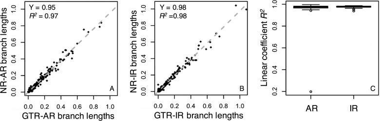
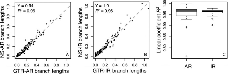
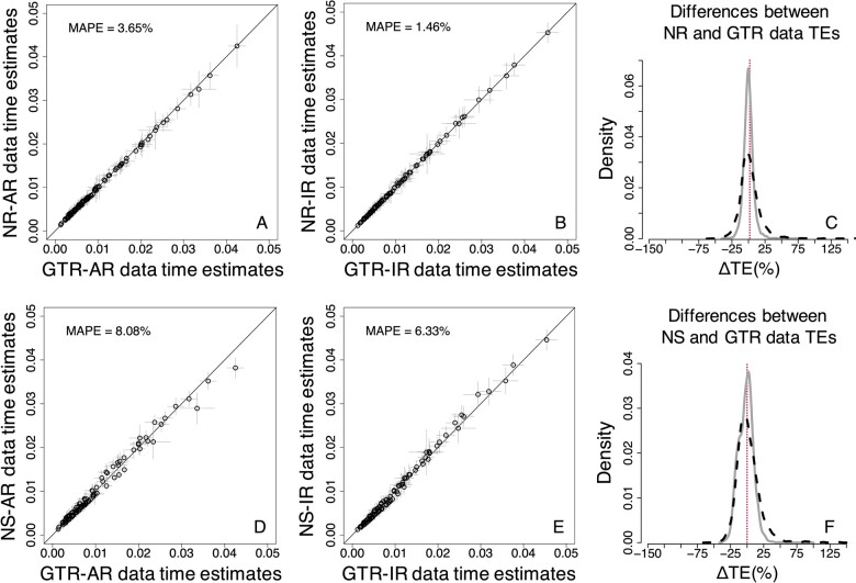
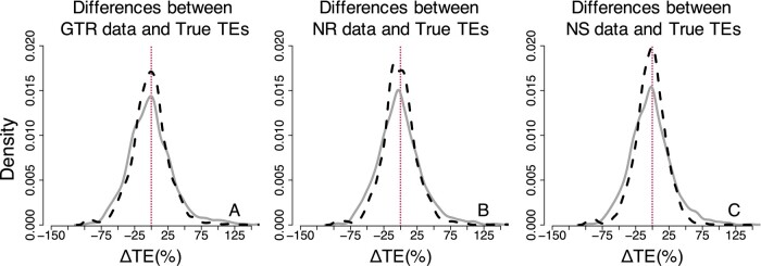
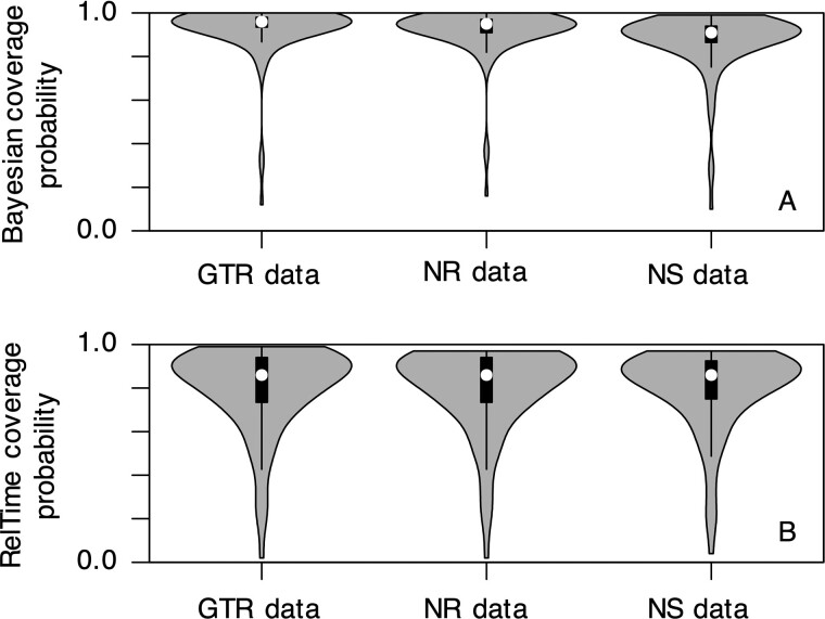
Results: We quantified the bias on time estimates that resulted from using the GTR + Γ model for the analysis of computer-simulated nucleotide sequence alignments that were evolved with non-stationary (NS) and non-reversible (NR) substitution models. We tested Bayesian and RelTime approaches that do not require a molecular clock for estimating divergence times. Divergence times obtained using a GTR + Γ model differed only slightly (∼3% on average) from the expected times for NR datasets, but the difference was larger for NS datasets (∼10% on average). The use of only a few calibrations reduced these biases considerably (∼5%). Confidence and credibility intervals from GTR + Γ analysis usually contained correct times. Therefore, the bias introduced by the use of the GTR + Γ model to analyze datasets, in which the time-reversibility and stationarity assumptions are violated, is likely not large and can be reduced by applying multiple calibrations.

Availability and implementation: All datasets are deposited in Figshare: https://doi.org/10.6084/m9.figshare.12594638.

Fig. 1.

A survey of substitution models selected in 141 research articles that published timetrees in year 2015–2017. More than 130 studies (>98%) used models that have more free parameters than the K80 model. All studies assumed stationarity and time-reversiblity of evolutionary processes, with the GTR + Γ and GTR + Γ+I being the most preferred models. K80, HKY, TrN and GTR represent Kimura-2-parameter (Kimura, 1980), Hasegawa–Kishino–Yano (Hasegawa et al., 1985), Tamura–Nei (Tamura and Nei, 1993) and GTR model (Tavaré, 1986), respectively. Model  + Γ(+I) means that either a gamma distribution for incorporating rate variation across sites is used, or a proportion of sites are assumed to be invariant across sequences, or both are used along with the corresponding substitution model

Fig. 2.

Phylogeny of 100 taxa showing calibrated nodes. The tree has been scaled to time on the basis of TEs from the Timetree of Life (Hedges and Kumar, 2009). Calibrations are represented for three nodes (red dots). We used a uniform distribution U(min, max) for the three calibrations: (1) root calibration U(444.6, 464.6); (2) Calibration-2 U(166.2, 186.2); (3) Calibration-3 U(157, 177). For the NS alignments, a NS process was added by changing the base composition and rate matrix for two lineages, starting at the ascending branches of node 2 (mGTR2) and node 3 (mGTR3)

Fig. 3.

A flowchart showing an overview of the simulation procedure used to generate datasets. We generated 150 alignments of 100 taxa from 50 phylogenies simulated using the AR model (50 GTR, 50 NR, and 50 NS) and 150 alignments from 50 phylogenies simulated using the IR model (50 GTR, 50 NR, and 50 NS)

Fig. 4.

Comparison of Bayesian TEs obtained by using the GTR + Γ model for analyzing GTR (model-match) and NR (model-mismatch) datasets simulated (A) with rate autocorrelation, AR, and (B) without rate autocorrelation, IR. Each data point represents the average of normalized times from 50 simulations (±1 SD—gray line). The MAPE is shown in the upper left corner of these panels. The black 1:1 line shows the trend if the estimates were equal. (C) Distributions of the normalized differences between GTR and NR data TEs for AR (black-dashed curve) and IR (gray curve) branch rates. For visual clarity, the distribution in (C) was truncated, removing a few outliers

Fig. 5.

Distributions of the normalized differences between estimated and true node times for GTR, NR, and NS datasets—Bayesian approach (root calibration only). Comparisons of AR (black-dashed curve) and IR (gray curve) performance for (A) GTR, (B) NR and (C) NS datasets. For visual clarity, the distribution in (A–C) was truncated, removing a few outliers

Fig. 6.

Comparison of RelTime estimates obtained by using the GTR + Γ model for GTR (model-match) and NR (model-mismatch) datasets simulated (A) with rate autocorrelation, AR, and (B) without rate autocorrelation, IR. Each data point represents the average of normalized times from 50 simulations (±1 SD—gray line). The MAPE is shown in the upper left corner of these panels. The black 1:1 line shows the trend if the estimates were equal. (C) Distributions of the normalized differences between GTR and NR TEs for AR (black-dashed curve) and IR (gray curve) datasets. For visual clarity, distribution in (C) was truncated, removing a few outliers

Fig. 7.

Branch length comparisons for GTR and NR datasets. Branch lengths were inferred by using the GTR + Γ model for (A) an AR dataset and (B) an IR dataset simulated under the GTR model (x-axis, model-match case) and the NR model (y-axis, model-mismatch case). They all show good linear relationships. The gray-dashed line is the best-fit linear regression through the origin. The slope (Y) and coefficient of determination (R²) are shown. (C) The dispersion of the linear trends of branch lengths. Boxes show the variation of the coefficient of determination of the linear regression (through the origin, R²) between branch lengths inferred using the GTR + Γ model for 50 GTR and 50 NR datasets simulated under AR and IR scenarios

Fig. 8.

Comparison of Bayesian TEs obtained by using the GTR + Γ model for GTR (model-match) and NS (model-mismatch) datasets simulated (A) with rate autocorrelation, AR, and (B) without rate autocorrelation, IR. Each data point represents the average of normalized times from 50 simulations (±1 SD—gray line). The MAPE is shown in the upper left corner of these panels. The black 1:1 line shows the trend if the estimates were equal. (C) Distributions of the normalized differences between GTR and NS data TEs for AR (black-dashed curve) and IR (gray curve) datasets. For visual clarity, the distribution in (C) was truncated, removing a few outliers

Fig. 9.

Comparison of TEs obtained by using the GTR + Γ model for GTR and NS datasets—RelTime approach (root calibration only). (A) AR datasets. (B) IR datasets. Each data point represents the average of normalized times from 50 simulations (±1 SD—gray line). The MAPE is shown in the upper left portion of each plot. The black line represents equality between estimates. (C) Distributions of the normalized differences between GTR and NS TEs for AR (black-dashed curve) and IR (gray curve) datasets. For visual clarity, the distribution in (C) was truncated, removing a few outliers

Fig. 10.

Branch lengths comparisons between GTR and NS data. Branch lengths inferred using the GTR + Γ model for (A) an AR dataset and (B) an IR dataset simulated under the GTR model (x-axis, model case) and the NS model (y-axis, model case) show a good linear relationship. The gray-dashed line is the best-fit linear regression through the origin. The slope (Y) and coefficient of determination (R²) are shown. (C) The dispersion of the linear trends of branch lengths. Boxes show the variation of the coefficient of determination of the linear regression (through the origin, R²) between branch lengths inferred using the GTR + Γ model for 50 GTR and 50 NS datasets simulated under AR and IR scenarios

Fig. 11.

Comparison of TEs obtained by using the GTR + Γ model for GTR, NR, and NS datasets—Bayesian approach (three calibrations). (A–C) NR datasets. (D–F) NS datasets. (A, B, D, and E) Each data point represents the average of normalized times from 50 simulations (±1 SD—gray line), generated using. The MAPE is shown in the upper left portion of each plot. The black line represents equality between estimates. Distributions of the normalized differences (C) between GTR and NR TEs, and (F) between GTR and NS TEs for AR (black-dashed curve) and IR (gray curve) datasets. For visual clarity, the distribution in (C) and (F) was truncated, removing a few outliers

Fig. 12.

Distributions of the normalized differences between estimated and true times on nodes for GTR, NR, and NS datasets—Bayesian approach (three calibrations). Comparisons of AR (black-dashed curve) and IR (gray curve) performance for (A) GTR, (B) NR, and (C) NS datasets. For visual clarity, the distribution in (A–C) was truncated, removing a few outliers

Fig. 13.

Comparison of TEs obtained by using the GTR + Γ model for GTR, NR and NS datasets—RelTime approach (three calibrations). (A–C) NR datasets. (D–F) NS datasets. (A, B, D, and E) Each data point represents the average of normalized times from 50 simulations (±1 SD—gray line). The MAPE is shown in the upper left portion of each plot. The black line represents equality between estimates. Distributions of the normalized differences (C) between GTR and NR TEs, and (F) between GTR and NS TEs for AR (black-dashed curve) and IR (gray curve) datasets. For visual clarity, the distribution in (C) and (F) was truncated, removing a few outliers

Fig. 14.

Distributions of the normalized differences between estimated and true times on nodes for GTR, NR, and NS datasets—RelTime approach (three calibrations). Comparisons of AR (black-dashed curve) and IR (gray curve) performance for (A) GTR, (B) NR, and (C) NS datasets. For visual clarity, the distribution in (A–C) was truncated, removing a few outliers

Fig. 15.

Distributions of coverage probabilities of all the nodes for GTR, NR, and NS datasets. Coverage probability of (A) Bayesian HPDs and (B) RelTime CIs for each scenario is calculated using results of 50 IR and 50 AR simulated datasets obtained using the GTR + Γ model and three calibrations. White dot represents the median value

References

1. Arenas M. (2015) Trends in substitution models of molecular evolution. Front. Genet., 6, 319. - PMC - PubMed
1. Blanquart S., Lartillot N. (2006) A Bayesian compound stochastic process for modeling non-stationary and non-homogeneous sequence evolution. Mol. Biol. Evol., 23, 2058–2071. - PubMed
1. Blanquart S., Lartillot N. (2008) A site- and time-heterogeneous model of amino acid replacement. Mol. Biol. Evol., 25, 842–858. - PubMed
1. dos Reis M., Yang Z. (2011) Approximate likelihood calculation on a phylogeny for Bayesian Estimation of Divergence Times. Mol. Biol. Evol., 28, 2161–2172. - PubMed
1. Fletcher W., Yang Z. (2009) INDELible: a flexible simulator of biological sequence evolution. Mol. Biol. Evol., 26, 1879–1888. - PMC - PubMed
Publication types