Asymmetries in visual acuity around the visual field

Abstract

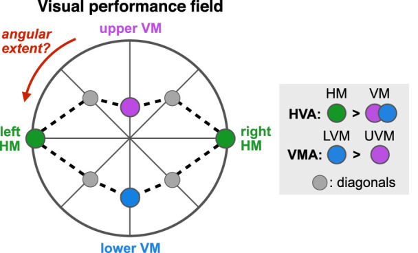
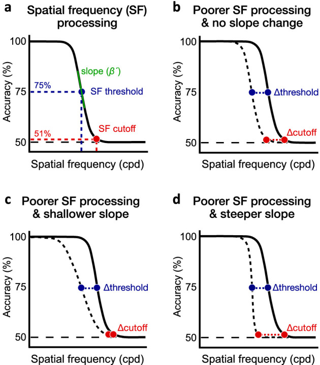
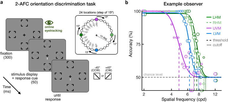
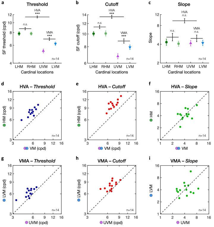
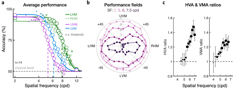
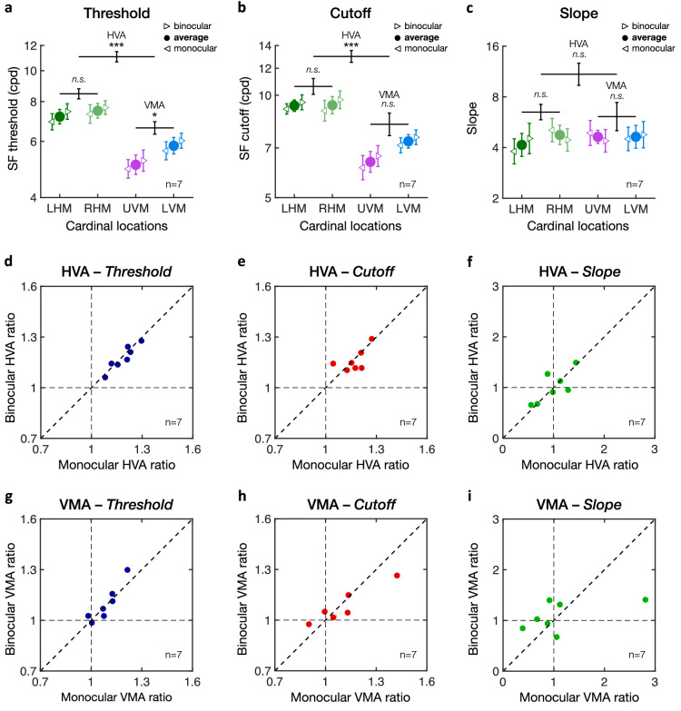
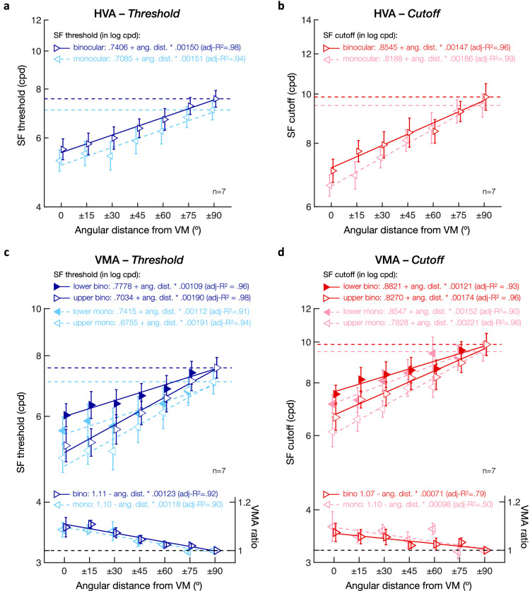
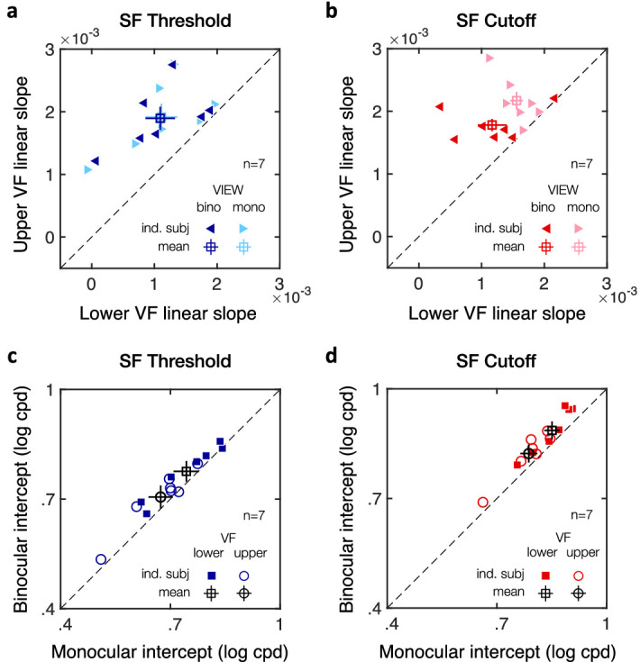
Human vision is heterogeneous around the visual field. At a fixed eccentricity, performance is better along the horizontal than the vertical meridian and along the lower than the upper vertical meridian. These asymmetric patterns, termed performance fields, have been found in numerous visual tasks, including those mediated by contrast sensitivity and spatial resolution. However, it is unknown whether spatial resolution asymmetries are confined to the cardinal meridians or whether and how far they extend into the upper and lower hemifields. Here, we measured visual acuity at isoeccentric peripheral locations (10 deg eccentricity), every 15° of polar angle. On each trial, observers judged the orientation (± 45°) of one of four equidistant, suprathreshold grating stimuli varying in spatial frequency (SF). On each block, we measured performance as a function of stimulus SF at 4 of 24 isoeccentric locations. We estimated the 75%-correct SF threshold, SF cutoff point (i.e., chance-level), and slope of the psychometric function for each location. We found higher SF estimates (i.e., better acuity) for the horizontal than the vertical meridian and for the lower than the upper vertical meridian. These asymmetries were most pronounced at the cardinal meridians and decreased gradually as the angular distance from the vertical meridian increased. This gradual change in acuity with polar angle reflected a shift of the psychometric function without changes in slope. The same pattern was found under binocular and monocular viewing conditions. These findings advance our understanding of visual processing around the visual field and help constrain models of visual perception.

Figure 1.

Graphic illustration of a canonical visual performance field (based on data from Carrasco et al., 2001). Each dot represents performance as a function of polar angle at a fixed eccentricity. The center of the polar plot corresponds to chance level, with highest performance typically observed along the horizontal meridian (HM; green), without differences between left and right hemifields. The horizontal-vertical anisotropy (HVA) depicts better performance in many tasks along the HM than the vertical meridian (VM). Moreover, performance is better at the lower VM (LVM; blue) than at the upper VM (UVM; purple), which is referred to as the vertical meridian asymmetry (VMA). Performance along the intercardinal (± 45°) meridians (gray) is usually similar, raising questions about the degree of visual performance fields as a function of polar angle.

Figure 2.

Spatial frequency (SF) processing. (a) Performance in SF discrimination decreases as stimulus SF increases. For each polar angle location, we estimated the 75%-correct SF threshold (blue dot) and SF cutoff (red dot) corresponding to the SF at which participants were near chance level (i.e., 51% correct). We also estimated the slope (β) of the psychometric function, which was converted into the maximum slope estimate (β´) (see Methods). (b) Differences in SF processing between two locations (e.g., UVM and LVM) could reflect a shift of the psychometric function without a change in slope. Such change would result in a similar difference in SF threshold and SF cutoff. (c, d) Asymmetries in SF processing could also be characterized by a change in the slope of the psychometric function. Relative to a similar change in SF threshold in both panels, a (c) shallower or (d) steeper slope would result in the change in SF cutoff to be less or more pronounced, respectively.

Figure 3.

(a) Trial sequence. Observers were asked to maintain fixation at the center of the screen, which was ensured using online eye-tracking. In a given session, grating stimuli were presented at four isoeccentric (10 deg eccentricity) locations. Observers were asked to report the orientation of the target stimulus at the location indicated by the response cue. Spatial frequency (SF) varied across trials. A total of 24 isoeccentric locations were tested across separate blocks by rotating the angular position of the 4 stimulus locations by 15°. The size of the placeholders, fixation point, and response cue have been enlarged for illustration purposes. (b) Example observer. Psychometric functions for one observer at the four cardinal locations (LHM/RHM = left/right horizontal meridian; UVM/LVM = upper/lower vertical meridian). Vertical dashed lines indicate the 75%-correct SF thresholds, and the dotted lines indicate SF cutoff estimates. The SF range used for each observer and location was adjusted between sessions to capture the dynamic range of the psychometric function. The size of each data point varies with the number of trials collected at each SF level.

Figure 4.

Horizontal vertical anisotropy (HVA) and vertical meridian asymmetry (VMA). Averaged binocular (a) SF threshold, (b) SF cutoff, and (c) slope estimates at each of the four cardinal locations (LHM = left horizontal meridian; RHM = right horizontal meridian; UVM = upper vertical meridian; LVM = lower vertical meridian). There was no difference between the LHM and RHM. The HVA corresponds to the difference between the HM (LHM and RHM combined) and VM (LVM and UVM combined). The VMA corresponds to the difference between the LVM and UVM. Error bars in panels a to c correspond to ± 1 SEM for each of the cardinal data points. Horizontal lines reflect comparisons between the LHM and RHM, between the HM and VM (i.e., HVA), and between the UVM and LVM (i.e., VMA), with error bars representing ± 1 SE of the mean difference. *p < 0.05, **p < 0.01, ***p < 0.001. (d–f) Scatterplots of individual participants' HVA for (d) threshold, (e) cutoff, and (f) slope estimates. (g–i) Scatterplots of individual participants' VMA for (g) threshold, (h) cutoff, and (i) slope estimates. Dots above the diagonal line indicate participants showing typical HVA and VMA patterns, which are observed for SF threshold and SF cutoff estimates but not for slope.

Figure 5.

Lack of correlation between the HVA and VMA. HVA and VMA ratios estimated from (a) SF threshold estimates or (b) SF cutoff estimates. Each data point corresponds to an individual participant's HVA and VMA ratios, with the solid black lines corresponding to Pearson correlations.

Figure 6.

No left-right hemifield difference. Changes in (a) SF threshold and (b) SF cutoff as a function of polar angle for the left and right hemifields. Polar plots of hemifields (left panels) show group-averaged SF estimates as a function of polar angle for the left and right hemifield locations separately (the data points corresponding to the UVM and LVM are color-coded as in Figure 1). Right panels show the same data with error bars corresponding to ± 1 SEM. No difference was observed between the left and right visual field (VF) locations. The asymmetry with polar angle between lower (−90° to 0°) and upper (0° to +90°) VF locations is characteristic of the VMA (HM = horizontal meridian; UVM/LVM = upper and lower vertical meridians).

Figure 7.

Angular extent of asymmetries in visual acuity. Group-averaged (a, c) SF threshold and (b, d) SF cutoff estimates plotted as a function of the angular distance from the vertical meridian (VM). Dashed line represents the value at the horizontal meridian (HM; green filled dot). (a, b) Horizontal vertical anisotropy (HVA). SF estimates were averaged across upper and lower hemifields, with the difference from the HM at 0° angular distance from the VM corresponding to the HVA. (c, d) Vertical meridian asymmetry (VMA). SF estimates plotted separately for the upper VF (open circles) and lower VF (filled circles), with the upper-lower difference at 0° angular distance from the VM corresponding to the VMA. VMA ratios plotted at the bottom of panels c and d were computed by dividing the lower by the upper visual field estimates. Adjusted R² values indicate the goodness of fit of linear regression equations. Error bars correspond to ± 1 SEM.

Figure 8.

Individual linear slope estimates from the linear mixed-effects models. Scatterplots of individual linear slope estimates with angular distance from the VM show a steeper linear slope in the upper than lower visual field (VF) in all participants (n = 14), for both (a) SF threshold and (b) SF cutoff estimates. Filled circles correspond to individual participants and the open square symbol to the mean ± 1 SEM.

Figure 9.

Impact of stimulus SF on performance fields. (a) Group-averaged orientation discrimination performance plotted as a function of the stimulus SF at the four cardinal locations (LHM/RHM = left/right horizontal meridian; UVM/LVM = upper/lower vertical meridian). Performance decreases similarly with increasing SF at the LHM and RHM locations, resulting in similar psychometric functions along the HM. Relative to the HM, performance at the VM is worse (i.e., HVA). Moreover, performance at the UVM location is poorer than at the LVM location (i.e., VMA). These asymmetries in SF processing reflected shifts of the psychometric functions without change in slope. Marker size indicates the number of participants averaged for each data point, which was restricted to a minimum of 4 out of the 14 participants. (b) Polar plot showing group-averaged performance as a function of the stimulus polar angle and SF, with the center of the polar plot corresponding to chance level (50% accuracy). Asymmetries at isoeccentric locations become more pronounced as stimulus SF increases. (c) Both the HVA and VMA performance ratios increase with stimulus SF. Each data point is the average performance ratio (± 1 SEM) computed at different stimulus SF within the dynamic range of the psychometric functions. Marker size indicates the number of participants averaged for each data point (varying from 4 to 14 participants).

Figure 10.

HVA and VMA under binocular and monocular viewing conditions. Averaged (a) SF threshold, (b) SF cutoff, and (c) slope estimates at each of the four cardinal locations (LHM/RHM = left/right horizontal meridian; UVM/LVM = upper/lower vertical meridian). Leftward and rightward triangles correspond to the monocular and binocular viewing condition, respectively. Filled circles correspond to average estimates across viewing conditions. Error bars correspond to ± 1 SEM. Horizontal lines reflect comparisons between the LHM and RHM, between the HM and VM (i.e., HVA), and between the UVM and LVM (i.e., VMA) for the combined binocular-monocular average data points, with error bars representing ± 1 SE of the mean difference. *p < 0.05, **p < 0.01, ***p < 0.001. (d–f) Scatterplots of individual participants’ HVA ratios (HM/VM) for (a) SF threshold, (b) SF cutoff, and (c) slope estimates. (g–i) Scatterplots of individual participants’ VMA ratios (LVM/UVM) for (g) SF threshold, (h) SF cutoff, and (i) slope estimates.

Figure 11.

Angular extent of visual asymmetries under monocular and binocular viewing conditions. (a, b) SF threshold and (b, d) SF cutoff estimates plotted as a function of the angular distance from the vertical meridian (VM). (a, b) HVA extent. SF estimates were computed for monocular (leftward triangles; dashed lines) and binocular (rightward triangles; solid lines) viewing conditions by averaging values at upper and lower visual field locations. (c, d) VMA extent. SF estimates for monocular (leftward triangles; dashed lines) and binocular (rightward triangles; solid lines), plotted separately for upper (open triangles) and lower (filled triangles) visual field locations. VMA ratios at the bottom of panels c and d were computed by dividing the lower by the upper visual field estimates for monocular and binocular viewing conditions separately. Linear regression equations and adjusted R² are provided for each linear fit. Error bars correspond to ± 1 SEM. Horizontal dashed lines represent values at the horizontal meridian.

Figure 12.

Individual estimates from the linear mixed-effects models. (a, b) Scatterplots of individual linear slope estimates with angular distance from the VM show steeper linear slope in the upper than lower visual field (VF), for both (a) SF threshold and (b) SF cutoff estimates. (c, d) Scatterplots of individual intercept estimates show higher SF intercepts under binocular than monocular viewing condition, for both (c) SF threshold and (d) SF cutoff estimates. Filled symbols correspond to individual participants (n = 7) and the open square symbols to the mean ± 1 SEM.

References

1. Abrams J., Nizam A., & Carrasco M. (2012). Isoeccentric locations are not equivalent: the extent of the vertical meridian asymmetry. Vision Research, 52(1), 70–78, 10.1016/j.visres.2011.10.016. - DOI - PMC - PubMed
1. Adams D. L., & Horton J. C. (2003). A precise retinotopic map of primate striate cortex generated from the representation of angioscotomas. Journal of Neuroscience, 23(9), 3771–3789, 10.1523/jneurosci.23-09-03771.2003. - DOI - PMC - PubMed
1. Akbas E., & Eckstein M. P. (2017). Object detection through search with a foveated visual system. PLoS Computational Biology, 13(10), e1005743, 10.1371/journal.pcbi.1005743. - DOI - PMC - PubMed
1. Altpeter E., Mackeben M., & Trauzettel-Klosinski S. (2000). The importance of sustained attention for patients with maculopathies. Vision Research, 40(10–12), 1539–1547, 10.1016/s0042-6989(00)00059-6. - DOI - PubMed
1. Anderson J. E., Cameron E. L., & Levine M. W. (2014). A method for quantifying visual field inhomogeneities. Vision Research, 105, 112–120, 10.1016/j.visres.2014.09.010. - DOI - PubMed
Publication types
LinkOut - more resources