. 2021 Jan;27(1):174-182.
doi: 10.1038/s41591-020-1142-7. Epub 2021 Jan 4.

A neuroimaging biomarker for sustained experimental and clinical pain

Affiliations

A neuroimaging biomarker for sustained experimental and clinical pain

Jae-Joong Lee et al. Nat Med. 2021 Jan.

Abstract

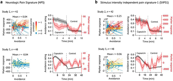
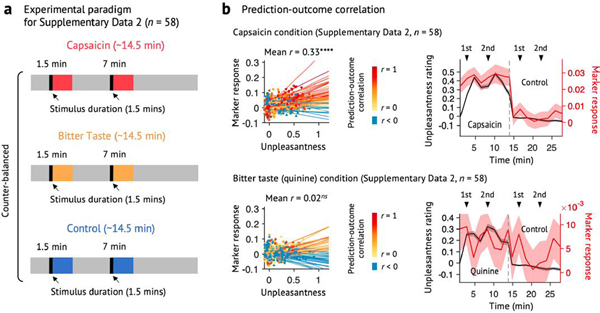
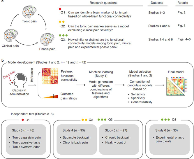
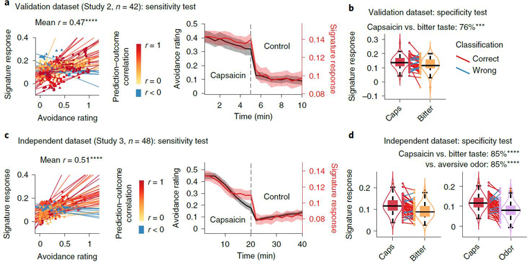
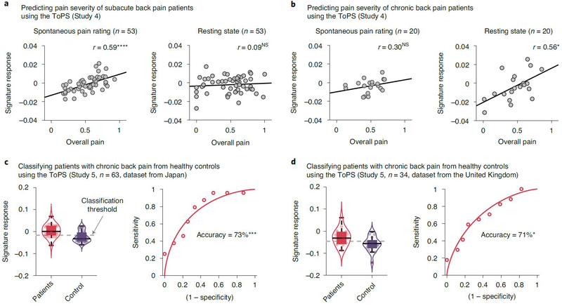
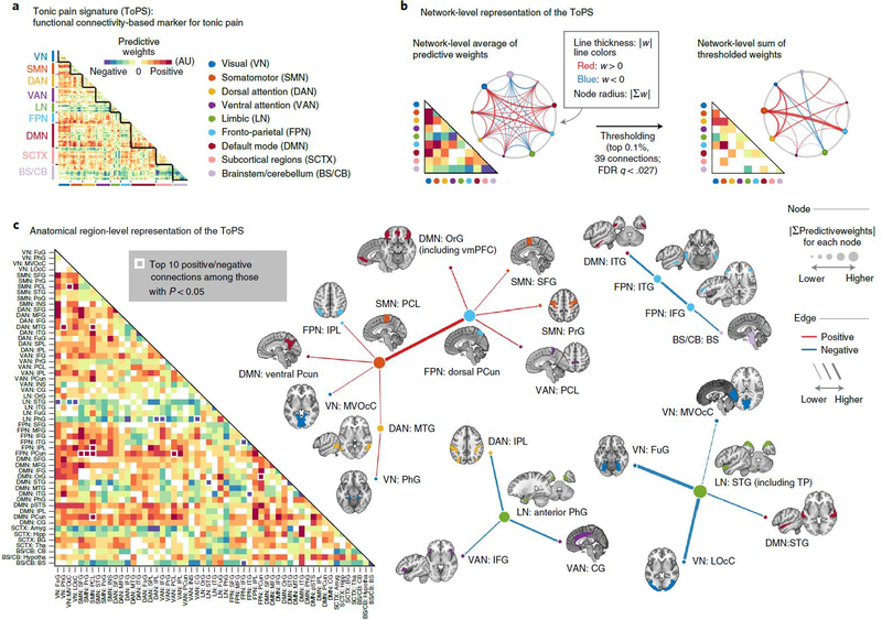
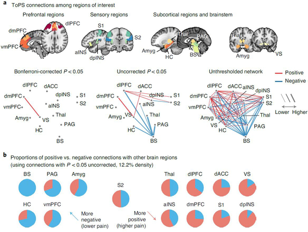
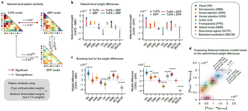
Sustained pain is a major characteristic of clinical pain disorders, but it is difficult to assess in isolation from co-occurring cognitive and emotional features in patients. In this study, we developed a functional magnetic resonance imaging signature based on whole-brain functional connectivity that tracks experimentally induced tonic pain intensity and tested its sensitivity, specificity and generalizability to clinical pain across six studies (total n = 334). The signature displayed high sensitivity and specificity to tonic pain across three independent studies of orofacial tonic pain and aversive taste. It also predicted clinical pain severity and classified patients versus controls in two independent studies of clinical low back pain. Tonic and clinical pain showed similar network-level representations, particularly in somatomotor, frontoparietal and dorsal attention networks. These patterns were distinct from representations of experimental phasic pain. This study identified a brain biomarker for sustained pain with high potential for clinical translation.


Conflict of interest statement

Competing interests

The authors declare no competing interests.

Figures

Extended Data Fig. 1 |
Extended Data Fig. 1 |. Behavioral data of Study 1.
a, Pain intensity and unpleasantness ratings of Study 1 (n = 19). b, Heart rate (HR; beat-per-minute) and skin conductance response (SCR; μS) of Study 1 (n = 14). Note that physiological data of five participants were discarded, because they were not recorded during scan or the data quality was too bad. Error bars represent within-subject standard errors of the mean (s.e.m.).
Extended Data Fig. 2 |
Extended Data Fig. 2 |. Overview of the signature development and test procedure.
Step 1: Model training. Using Study 1 data, we trained a large number of candidate models for each outcome variable (pain intensity and unpleasantness) with multiple combinations of different parcellation solutions (features), connectivity estimation methods (feature engineering), algorithms, and hyperparameters. We generated a total of 5916 candidate models for each outcome variable. Step 2: Model competition. To select the best model, we conducted a competition among the candidate models based on the pre-defined criteria including sensitivity, specificity, and generalizability based on cross-validated performance in Study 1 and also using Study 2 data as a validation dataset. For the full description of the competition procedure, please see Methods, and for the full report of the competition results, please see Extended Data Fig. 3. Step 3: Independent testing. To further characterize the final model in multiple test contexts, we tested the final model on multiple independent datasets, including two additional tonic pain dataset (Study 3 and Supplementary Data 2), three clinical pain datasets (Studies 4–5 and Supplementary Data 1), and one experimental phasic pain dataset (Study 6). Gray boxes represent locally collected datasets, and green boxes represent publicly available datasets. Different font colors indicate different scan sites.
Extended Data Fig. 3 |
Extended Data Fig. 3 |. Model competition results of pain intensity models.
Using multiple candidate models generated from the model development step (see Extended Data Fig. 2 and Methods for details), we conducted a model competition using 7 predefined criteria. The criteria consist of 4 correlation coefficients (within- and between-individual prediction-outcome correlations of Studies 1 and 2; shown in the top panel), and 3 classification accuracy values (for Capsaicin vs. Control in Studies 1 and 2, and for Capsaicin vs Quinine in Study 2; shown in the middle panel). Dotted lines separate different parcellations, and colored bars on the top of the plots (gray, light green, green, red, orange, and pink) represent different options of connectivity calculation methods and algorithms (see the top right for detailed description for each color bar). For CPM-based models (gray and red color bars), thresholds become more stringent from the left to the right. For PCR-based models (light green, green, orange, and pink), more PCs were used from the left to the right. To combine the 7 different performance metrics, we used a percentile-based scoring method (ranging from 0 to 100 for each criterion). The combined score (possible range: 0 to 700) was shown in the bottom panel, and the selected best model was indicated with the red arrow on the plots. Here we show the competition results only for the predictive model for pain intensity.
Extended Data Fig. 4 |
Extended Data Fig. 4 |. Specificity tests using a prediction approach (Study 3).
We used the ToPS to predict the avoidance ratings while participants were given a, bitter taste (quinine) or b, aversive odor. Left: Actual versus predicted ratings (that is, signature response) are shown in the plot. Signature response was calculated using the dot product of the model with the data. Signature response is using an arbitrary unit. Each colored line (or symbol) represents an individual participant’s data for across the treatment (quinine or aversive odor) and control runs (red: higher r, yellow: lower r, blue: r < 0). The exact P-values were P = 0.014 for bitter taste and P = 0.372 for aversive odor, two-tailed, bootstrap tests, n = 48. Right: Mean avoidance rating (black) and signature response (red) across the treatment and control runs. Shading represents within-subject s.e.m. Note that the left and right plots were based on averaging within five and ten time bins, respectively. ns = non-significant, *P < 0.05.
Extended Data Fig. 5 |
Extended Data Fig. 5 |. Noise analysis.
a, Univariate comparisons of head motion (framewise displacement, FD) and physiological measures (heart rate, HR, and respiratory rate, RR) between the capsaicin versus control conditions with the independent test dataset (Study 3, n = 48). We used the violin and box plots to show the distributions of the values. The box was bounded by the first and third quartiles, and the whiskers stretched to the greatest and lowest values within median ±1.5 interquartile range. The data points outside of the whiskers were marked as outliers. Note that 10 participants’ physiological data were excluded due to technical issues with acquisition (remaining n = 38). For statistical testing, paired t-tests (two-tailed) were conducted. b, Noise analysis 1. To examine whether the nuisance and physiology variables explain the Tonic Pain Signature (ToPS) response, we trained a model to predict the ToPS scores based on 34 nuisance variables + 2 additional physiology variables with Study 3 data. The 34 nuisance variables included 24 head motion parameters (6 movement parameters including x, y, z, roll, pitch, and yaw, their mean-centered squares, their derivatives, and squared derivative), 5 principal component scores derived from white matter (WM), and 5 principal component scores derived from cerebrospinal fluid (CSF). The 2 physiological variables were heart rate and respiratory rate. Because the effects of these confounding variables can be different across individuals and conditions, we trained predictive models for each condition and for each individual. To achieve more stable and unbiased predictive performance, we divided the data into 40 time-bins (each bin was 30 seconds) and conducted 10-fold cross-validation. Prediction-outcome correlation coefficients are visualized with violin and box plots. For statistical testing, we used one-sample t-test, two-tailed. c, Noise analysis 2. To test whether the ToPS responses can explain tonic pain ratings above and beyond the nuisance and physiology variables, we conducted multi-level general linear model (GLM) analysis (n = 38) using data averaged within 10 time bins for each individual across capsaicin and control condition (5 bins per condition), which is the same binning scheme as our main prediction results (Fig. 2c). To obtain standardized beta coefficients, all the features were z-scored. The exact P-values were (from left to right) 1.86 × 10⁻⁸ (ToPS), 0.231 (FD), 0.145 (mean WM), 0.270 (mean CSF), 0.270 (HR), and 0.272 (RR), two-tailed, multi-level GLM with bootstrap tests, 10,000 iterations. Overall, participants moved more and showed heart-rate acceleration during capsaicin (a), but the ToPS model was independent of movement and physiological variables (b). ToPS predicted pain avoidance ratings controlling for movement and physiological nuisance variables, but the nuisance variables themselves did not predict avoidance ratings. ns = not significant; ****P < 0.0001.
Extended Data Fig. 6 |
Extended Data Fig. 6 |. Predictive performance of the clinical pain models.
a, Predictive performance of the SBP model, which was derived using a half of SBP patients’ spontaneous pain rating task data (n = 35, training set). The SBP model was then tested on the remaining half of the SBP data (n = 35, hold-out test set) to obtain an unbiased estimate of the predictive performance. Leave-one-subject-out cross-validation was used for predicting pain scores within the training dataset. The exact P-values for the prediction performance was 0.0002 for the training set (left) and 0.032 for the hold-out test set (right), two-tailed, one-sample t-test. b, Cross-validated performance of the CBP model, which was derived using the whole CBP patients’ resting state data (n = 17, after excluding data with insufficient brain coverages). Because the CBP model showed poor predictive performance even within the training dataset, further testing of the CBP model was discontinued. The exact P-value of the prediction performance was P = 0.269, two-tailed, one-sample t-test). ns = not significant, *P < 0.05, ***P < 0.001.
Extended Data Fig. 7 |
Extended Data Fig. 7 |. Circular plot representation of the ToPS.
From outermost to innermost, the first layer of the circle represents different functional groups, and the second and third layers each represent the sum of positive and negative predictive weights coming from each brain region.
Extended Data Fig. 8 |
Extended Data Fig. 8 |. Ventral striatum seed-based connectivity analysis.
a, We used the bilateral ventral striatum (VS) ROIs from the ToPS model as a seed to construct whole-brain seed-based connectivity maps for each time-bin of Study 1 data (n = 19). We had a particular interest in the weight patterns within the two medial prefrontal regions, dorsomedial and ventromedial prefrontal cortices (dmPFC and vmPFC). With the whole-brain connectivity maps, b, we first conducted the univariate GLM analysis. For each individual, we regressed the VS seed-based functional connectivity (Y) on pain intensity ratings (X) across capsaicin and control runs and performed second-level t-tests on the beta maps, treating participant as a random effect. Here we show the results for FDR-corrected q < 0.05 (corresponding to uncorrected P = 0.001), pruned with uncorrected P < 0.01 and 0.05 (two-tailed). c, We also conducted a multivariate analysis, in which we used the principal component regression (PCR) with reduced number of PCs to predict pain intensity ratings based on VS seed-based connectivity across capsaicin and control condition. The number of PCs was selected based on cross-validated within-individual predictive performance (#PC = 45; mean prediction-outcome r = 0.25, P = 0.002, two-tailed, bootstrap test). To identify important brain regions, we conducted the bootstrap test for the PCR with 10,000 iterations. Here we show the results for P < 0.005 uncorrected, pruned with P < 0.01 and 0.05, two-tailed. d, Regression weights in the medial prefrontal regions, focusing on the dorsomedial and ventromedial prefrontal cortices (that is, dmPFC and vmPFC). The left panel shows the unthresholded univariate map from b, and the right panel shows the unthresholded multivariate regression map from c. The pie chart represents the proportion of positive (red) and negative (blue) weights in each of the medial prefrontal regions. Across both univariate and multivariate maps, a dorsal-ventral gradient (dorsal: more positive, ventral: more negative) was found in the medial prefrontal cortex. Black lines show the contours of dmPFC and vmPFC regions.
Extended Data Fig. 9 |
Extended Data Fig. 9 |. Predicting tonic pain ratings with fMRi activation-based signatures for EPP.
To examine whether the fMRI activation-based pain markers could achieve similar levels of predictive performance, we tested existing fMRI activation-based models, including a, the Neurologic Pain Signature (NPS) and b, the Stimulus Intensity Independent Pain Signature-1 (SIIPS1). The top panel shows the predictive performances on the validation dataset (Study 2), and the bottom panel shows the predictive performances on the independent dataset (Study 3). In the plots on the left-side, the color of dots and lines represented the levels of correlation (r) for each participant’s pain prediction (red: higher r; yellow: lower r, blue: r < 0). The plots on the right-side show mean values of the actual avoidance ratings (black) and signature responses (red). The capsaicin run was shown before the control run for the display purpose, and in the real experiment, the order of the runs was counterbalanced across participants. Shading represents the standard errors of the mean (s.e.m.). Note that the left and right plots were based on averaging within five and ten time bins, respectively.
Extended Data Fig. 10 |
Extended Data Fig. 10 |. Testing the ToPS on an independent dataset with a different time-course of tonic pain and bitter taste (Supplementary Data 2).
We used the ToPS to predict the unpleasantness ratings while participants were given capsaicin, quinine (bitter taste), or saline (‘Control’). Here, the capsaicin and quinine stimuli were delivered to participants’ mouths using an MR-compatible gustometer system. This experimental setup allowed us to evoke capsaicin-induced orofacial tonic pain or quinine-induced bitter taste during two separate epochs within one run. a, Experimental paradigm for Supplementary Data 2 (n = 58). Each run lasts for around 14.5 minutes, and each stimulus (capsaicin for ‘Capsaicin’, quinine for ‘Bitter Taste’, and saline for ‘Control’ condition) was delivered two times within each run (1.5–3 min, and 7–8.5 min). The order of all conditions was counterbalanced across participants. b, Left: Actual versus predicted ratings (that is, signature responses) are shown in the plot. Signature response was calculated using the dot product of the model with imaging data. Each colored line (or symbol) represents an individual participant’s data across the capsaicin and control runs (red: higher r, yellow: lower r, blue: r < 0). Right: Mean avoidance rating (black) and signature response (red) across the capsaicin and control runs. Black arrows indicate when taste stimuli were delivered to participants. Shading represents within-subject s.e.m. The capsaicin and quinine runs are shown before the control run for the display purpose, regardless of the actual order of the two runs. Note that the left and right plots were based on averaging within five and ten time bins, respectively. The exact P-values were P = 3.32 × 10⁻⁹ for the capsaicin condition (top) and 0.710 for the bitter taste condition (bottom), two-tailed, bootstrap tests. ****P < 0.0001.
Fig. 1 |
Fig. 1 |. Overview of research questions and main analyses.
a, This study aims to answer the three research questions (Q1–3) using six independent datasets and the predictive modeling approach. b, Overview of the experiment and data analyses to answer the research questions. We acquired fMRI data while participants experienced tonic orofacial pain and generated many candidate models predictive of pain ratings based on the functional connectivity patterns during tonic pain experience (Study 1). The final model was selected through a model competition using a set of predefined criteria across training and validation datasets (Studies 1 and 2). We further validated the final model on prospective independent datasets (Studies 3–6). Different studies were used for answering different main research questions (for example, Study 3 for Q1, Studies 4 and 5 for Q2 and Study 6 for Q3).
Fig. 2 |
Fig. 2 |. Sensitivity and specificity test results.
We show the sensitivity and specificity of the ToPS on the validation dataset (Study 2, n = 42) and on an independent dataset (Study 3, n = 48). Note that the results based on the validation dataset in a and b are somewhat biased because the hyperparameters were optimized using this dataset, whereas the results in c and d are unbiased given that this dataset was held out for testing until the model was developed. To obtain rating scores on a same scale across different stimulus modalities, we used an avoidance rating scale (question: ‘How much do you want to avoid this experience in the future?’). a, Left: actual versus predicted ratings (that is, signature response) are shown in the plot. Signature response was calculated using the dot product of the model with the data and using an arbitrary unit. Each colored line (or symbol) represents individual participant’s data for across the capsaicin and control runs (red, higher r; yellow, lower r; blue, r < 0). P = 3.24 × 10⁻¹⁰, two-tailed, bootstrap test, n = 42. Right: mean avoidance rating (black) and signature response (red) across the capsaicin and control runs. Shading represents within-subject s.e.m. The capsaicin run is shown before the control run for the display purpose, regardless of the actual order of the two runs. Note that the left and right plots were based on averaging within five and ten time bins, respectively. b, We conducted a forced two-choice test to classify the mean signature response during the capsaicin run versus the bitter taste (quinine) run. We used the violin and box plots to show the distributions of the signature response. The box was bounded by the first and third quartiles, and the whiskers stretched to the greatest and lowest values within median ±1.5 interquartile range. The data points outside of the whiskers were marked as outliers. Each colored line between dots represents each individual participant’s paired data (red line, correct classification; blue line, incorrect classification). P = 0.0009, two-tailed, binomial test, n = 42. c, Left: actual versus predicted ratings. P = 3.20 × 10⁻¹⁴, two-tailed, bootstrap test, n = 48. Right: mean avoidance rating (black) and signature response (red) across the capsaicin and control runs. Shading represents within-subject s.e.m. d, A forced two-choice test results with two different test conditions, bitter taste and aversive odor conditions. P = 6.24 × 10⁻⁷ for both tests, two-tailed, binomial tests, n = 48. ***P < 0.001 and ****P < 0.0001, two tailed.
Fig. 3 |
Fig. 3 |. Testing the ToPS on the clinical pain data.
a, b, We tested the ToPS on a publicly available clinical pain dataset,– (Study 4) to evaluate how much the model can explain clinical pain severity of (a) patients with subacute back pain (SBP; n = 53) and (b) patients with chronic back pain (CBP; n = 20). The plots show the relationships between the actual pain scores (visual analog scale) versus signature response (arbitrary unit). Each dot represents an individual participant, and the line represents the regression line. The exact P values and degrees of freedom (d.f.) were (a) P = 3.91 × 10⁻⁶ (left) and 0.528 (right), d.f. = 51; (b) P = 0.197 (left) and 0.011 (right), d.f. = 18; two-tailed, one-sample t-test. c, d, We further tested the ToPS on two publicly available datasets to evaluate how well the model can classify the patients with CBP from healthy control participants. One dataset (c) was obtained from Japan (n = 63), which included 24 patients and 39 healthy participants. The other dataset (d) was obtained from the United Kingdom (n = 34), which included 17 patients and 17 healthy participants. The exact P values were P = 0.0003 for c and P = 0.024 for d, two-tailed, binomial tests. *P < 0.05, ***P < 0.001 and ****P < 0.0001. NS, not significant.
Fig. 4 |
Fig. 4 |. ToPS: a functional connectivity marker for tonic pain.
a, The raw predictive weights of the model. We sorted the brain regions according to their functional network membership. b, Left: we averaged the ToPS predictive weights for each network and displayed them with a lower triangular matrix and a circular plot. Right: we summed the top 0.1% thresholded weights based on bootstrap test with 10,000 iterations (P < 0.000028, FDR-corrected q < 0.027, two tailed) at the network level. c, We grouped the parcels into gross anatomical regions within each functional network and averaged the predictive weights within each anatomical region. The top ten positive and negative connections and the corresponding brain regions that survived at a threshold of uncorrected P < 0.05 with bootstrap tests (two tailed, white boxes on the left panel) were shown with force-directed graph layout. AU: arbitrary unit; Amyg, amygdala; BS, brainstem; BG, basal ganglia; CB, cerebellum; CG, cingulate gyrus; FuG, fusiform gyrus; Hipp, hippocampus; Hypotha, hypothalamus; IFG, inferior frontal gyrus; INS, insular gyrus; IPL, inferior parietal lobule; ITG, inferior temporal gyrus; LOcC, lateral occipital cortex; MFG, middle frontal gyrus; MTG, middle temporal gyrus; MVOcC, medioventral occipital cortex; OrG, orbital gyrus; PCL, paracentral lobule; PCun, precuneus; PhG, parahippocampal gyrus; PoG, postcentral gyrus; PrG, precentral gyrus; pSTS, posterior superior temporal sulcus; SFG, superior frontal gyrus; SPL, superior parietal lobule; STG, superior temporal gyrus; Tha, thalamus.
Fig. 5 |
Fig. 5 |. ToPS connections among ROis.
a, We examined the ToPS predictive weights among the ROIs that have been often studied in the field of pain neuroimaging, including prefrontal (vmPFC, dmPFC, dlPFC and dACC), sensory (S1, S2, aINS and dpINS), subcortical (thalamus, ventral striatum, amygdala and hippocampus) and brainstem (PAG and brainstem) regions. We displayed these connections with three different levels of threshold. Left: Bonferroni correction P < 0.05; middle: uncorrected P < 0.05; right: no threshold. P values were obtained from bootstrap tests with 10,000 iterations (two tailed). b, For each pain-related brain region, we show proportions of positive versus negative connections with other brain regions with pie charts (red. positive; blue, negative). We used only the connections that survived at a threshold of uncorrected P < 0.05 (bootstrap tests, two tailed) for calculating proportions. Brain regions with a higher proportion of negative connections are shown on the left side (meaning lower pain with increasing connectivity), and those with a higher proportion of positive connections are shown on the right side (meaning higher pain with increasing connectivity).
Fig. 6 |
Fig. 6 |. Comparing the ToPS with the SBP and ePP models.
The predictive weights of the ToPS were compared to functional connectivity-based models of SBP and EPP. a, Pattern similarity among three different pain models, calculated by taking Pearson’s correlation between the network-level average of unthresholded (UT; statistics above the line) or thresholded (T; statistics below the line) predictive weights. For thresholding, the top 0.1% stable connections based on bootstrap tests were selected. The exact P values between ToPS and SBP were P = 0.095 (UT) and 0.036 (T); between ToPS and EPP, P = 0.795 (UT) and 0.817 (T); between SBP and EPP, P = 0.747 (UT) and 0.940 (T), two-tailed, one-sample t-test, d.f. = 43. b, Network-level differences of predictive weights between different pain models; the closed circles indicate the mean network-level weights of the ToPS, and the open circles are for the SBP model (left) or the EPP model (right). Color represents different functional networks. c, Bootstrap test results (10,000 iterations) of the network-level weight differences between the ToPS versus SBP model (left) or EPP model (right). The exact P values for ToPS-SBP were (from left to right): 1.95 × 10⁻⁸ (VN), 0.728 (SMN), 0.021 (DAN), 0.009 (VAN), 1.05 × 10⁻⁵ (LN), 0.019 (FPN), 6.04 × 10⁻⁸ (DMN), 0.084 (SCTX) and 4.91 × 10⁻⁹ (BS/CB). For ToPS-EPP, P = 1.66 × 10⁻²² (VN), 0.0005 (SMN), 3.72 × 10⁻¹² (DAN), 0.904 (VAN), 2.77 × 10⁻¹⁷ (LN), 6.28 × 10⁻⁹ (FPN), 1.72 × 10⁻¹⁹ (DMN), 0.709 (SCTX) and 3.66 × 10−53 (BS/CB), two-tailed, bootstrap tests. d, Comparison of the network-level distance (absolute difference) between pain models. Each colored dot indicates the absolute network-level weight difference between the ToPS (wToPS) and bootstrapped SBP models (wSBP-boot; x axis) and bootstrapped EPP model (wEPP-boot; y axis). The error bars from the center dots represent the s.d. from the mean of the sampling distribution with bootstrap tests. The dashed line indicates y = x (that is, same distance from the ToPS). Seven of the nine functional networks were located above the dashed line, which indicates that the weight distance between the ToPS and the SBP model was shorter than the weight distance between the ToPS and the EPP model for these networks. +P < 0.05, one tailed; *P < 0.05, **P < 0.01, and ****P < 0.0001, two tailed. NS, not significant (for the significance in c, Bonferroni correction was used).

Comment in

References

    1. Dahlhamer J et al.Prevalence of chronic pain and high-impact chronic pain among adults - United States, 2016. MMWR Morb. Mortal. Wkly. Rep 67, 1001–1006 (2018). - PMC - PubMed
    1. Gaskin DJ & Richard P The economic costs of pain in the United States. J. Pain 13, 715–724 (2012). - PubMed
    1. Chapman CR & Gavrin J Suffering: the contributions of persistent pain. Lancet 353, 2233–2237 (1999). - PubMed
    1. Apkarian AV Pain perception in relation to emotional learning. Curr. Opin. Neurobiol 18, 464–468 (2008). - PMC - PubMed
    1. Hashmi JA et al.Shape shifting pain: chronification of back pain shifts brain representation from nociceptive to emotional circuits. Brain 136, 2751–2768 (2013). - PMC - PubMed

Publication types

MeSH terms

LinkOut - more resources