Extracting the dynamics of behavior in sensory decision-making experiments

Abstract

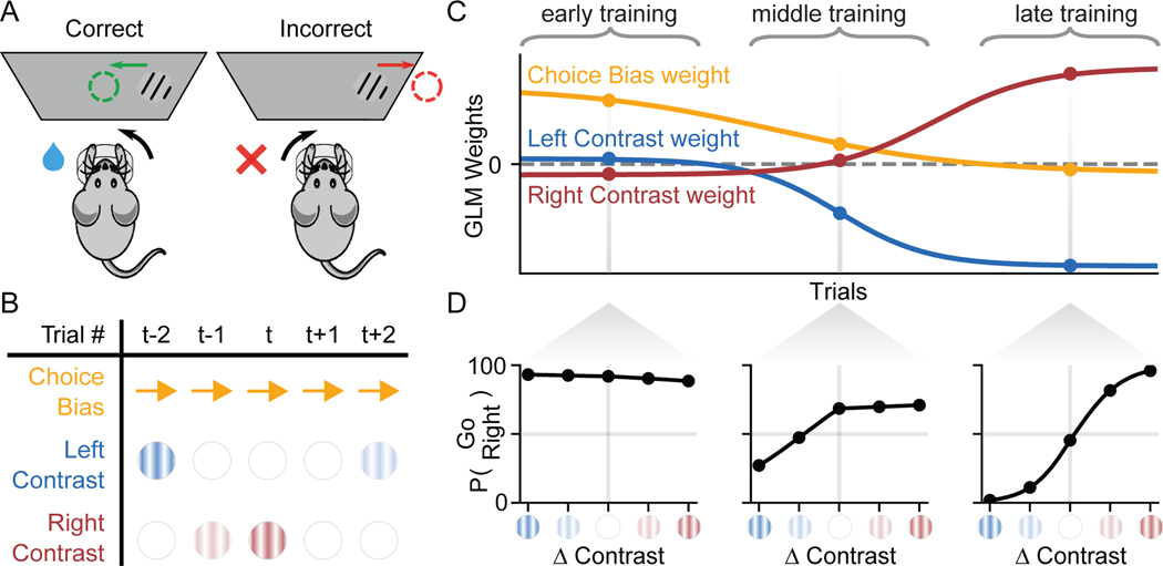
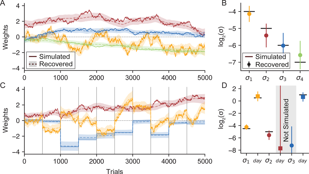
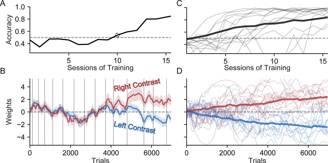
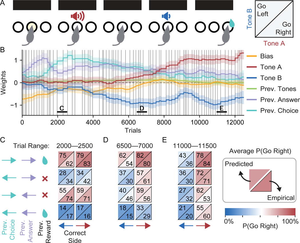
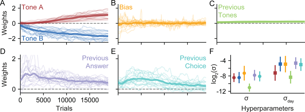
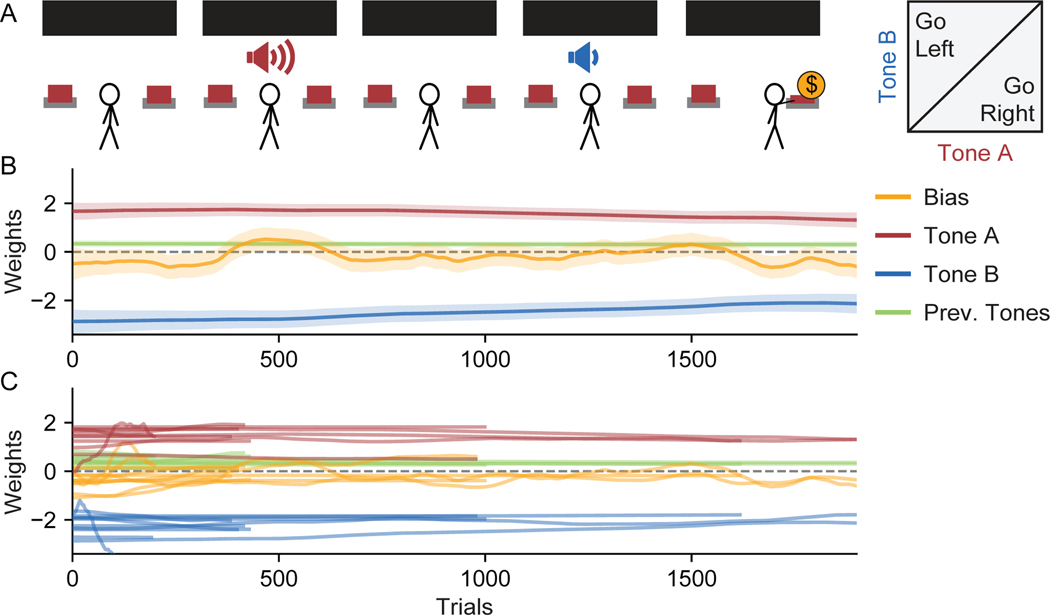
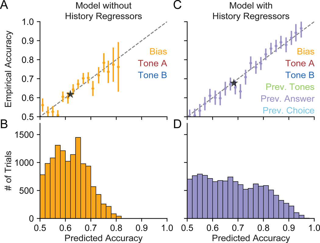
Decision-making strategies evolve during training and can continue to vary even in well-trained animals. However, studies of sensory decision-making tend to characterize behavior in terms of a fixed psychometric function that is fit only after training is complete. Here, we present PsyTrack, a flexible method for inferring the trajectory of sensory decision-making strategies from choice data. We apply PsyTrack to training data from mice, rats, and human subjects learning to perform auditory and visual decision-making tasks. We show that it successfully captures trial-to-trial fluctuations in the weighting of sensory stimuli, bias, and task-irrelevant covariates such as choice and stimulus history. This analysis reveals dramatic differences in learning across mice and rapid adaptation to changes in task statistics. PsyTrack scales easily to large datasets and offers a powerful tool for quantifying time-varying behavior in a wide variety of animals and tasks.

Keywords: behavioral dynamics; learning; psychophysics; sensory decision making.

Figure 1:

Schematic of Binary Decision-Making Task and Dynamic Psychophysical Model (A) A schematic of the IBL sensory decision-making task. On each trial, a sinusoidal grating (with contrast values between 0 and 100%) appears on either the left or right side of the screen. Mice must report the side of the grating by turning a wheel (left or right) in order to receive a water reward (see ar]STAR Methods for details) (IBL et al., 2020). (B) An example table of the task variables X assumed to govern behavior for a subset of trials {t − 2,…, t + 2}, consisting here of a choice bias (a constant rightward bias, encoded as “+1” on each trial), the contrast value of the left grating, and the contrast value of the right grating. (C) Hypothetical time-course of a set of psychophysical weights W, which evolve smoothly over the course of training. Each weight corresponds to one of the K = 3 variables comprising x_t, such that a weight’s value at trial t indicates how strongly the corresponding variable is affecting choice behavior. (D) Psychometric curves defined by the psychophysical weights w_t on particular trials in early, middle, and late training periods, as defined in (C). Initial behavior is highly biased and insensitive to stimuli (“early training”). Over the course of training, behavior evolves toward unbiased, high-accuracy performance consistent with a steep psychometric function (“late training”).

Figure 2:

Recovering Psychophysical Weights from Simulated Data (A) To validate PsyTrack, we simulated a set of K = 4 weights $\widehat{\mathbf{w}}$ that evolved for T = 5000 trials (solid lines). We then use our method to recover weights W (dashed lines), surrounded with a shaded 95% credible interval. The full optimization takes less than one minute on a laptop, see Figure S1 for more information. (B) In addition to recovering the weights W in (A), we also recovered the smoothness hyperparameter σ_k for each weight, also plotted with a 95% credible interval. True values ${\widehat{\sigma }}_k$ are plotted as solid black lines. (C) We again simulated a set of weights as in (A), except now session boundaries have been introduced at 500 trial intervals (vertical black lines), breaking the 5000 trials into 10 sessions. The yellow weight is simulated with a σ_day hyperparameter much greater than its respective σ hyperparameter, allowing the weight to evolve trial-to-trial as well as “jump” at session boundaries. The blue weight has only a σ_day and no σ hyperparameter meaning the weight evolves only at session boundaries. The red weight does not have a σ_day hyperparameter, and so evolves like the weights in (A). See Figure S2 for weight trajectories recovered for this dataset without the use of any σ_day hyperparameters. (D) We recovered the smoothness hyperparameters θ for the weights in (C). Though the simulation only has four hyperparameters, the model does not know this and so attempts to recover both a σ and a σ_day hyperparameter for all three weights. The model appropriately assigns low values to the two non-existent hyperparameters (gray shading).

Figure 3:

Visualization of Early Learning in IBL Mice (A) The accuracy of an example mouse over the first 16 sessions of training on the IBL task. We calculated accuracy only from “easy” high-contrast (50% and 100%) trials, since lower-contrast stimuli were only introduced later in training. The first session above chance performance (50% accuracy) is marked with a dotted circle. (B) Inferred weights for left (blue) and right (red) stimuli governing choice for the same example mouse and sessions shown in (A). Grey vertical lines indicate session boundaries. The black dotted line marks the start of the tenth session, when left and right weights first diverged, corresponding to the first rise in accuracy above chance performance (shown in (A)). See Figure S3 for models using additional weights. (C) Accuracy on easy trials for a random subset of individual IBL mice (gray), as well as the average accuracy of the entire population (black). (D) The psychophysical weights for left and right contrasts for the same subset of mice depicted in (C) (light red and blue), as well as the average psychophysical weights of the entire population (dark red and blue) (σ_day was omitted from these analyses for visual clarity).

Figure 4:

Adaptation to Bias Blocks in an Example IBL Mouse (A) An extension of Figure 3A to include the first months of training (accuracy is calculated only on “easy” high-contrast trials). Starting on session 17, our example mouse was introduced to alternating blocks of 80% right contrast trials (right blocks) and 80% left contrasts (left blocks). The sessions where these bias blocks were first introduced are outlined (pink), as are two sessions in later training where the mouse has adapted to the block structure (purple). Figure S5 validates model fits to sessions 10, 20, & 40 against psychometric curves generated directly from behavior. (B) Three psychophysical weights evolving during the transition to bias blocks, with right (left) blocks in red (blue) shading. Weights correspond to contrasts presented on the left (blue) and right (red), as well as a weight on choice bias (yellow). See Figure S4 for models that parametrize contrast values differently. (C) After several weeks of training on the bias blocks, the mouse learns to quickly adapt its behavior to the alternating block structure, as can be seen in the dramatic oscillations of the bias weight in sync with the blocks. (D) The bias weight of our example mouse during the first three sessions of bias block, where the bias weight is chunked by block and each chunk is normalized to start at 0. Even during the initial sessions of bias blocks, the red (blue) lines show that a mild rightward (leftward) bias tended to evolve during right (left) blocks. (E) Same as (D) for three sessions during the “Late Bias Blocks” period. Changes in bias weight became more dramatic, tracking stimulus statistics more rapidly, and indicating that the mouse had adapted its behavior to the block structure of the task. While some of the bias weight trajectories may appear to “anticipate” the start of the next block, this is largely an methodological artifact of the smoothing used in the model (see Figure S6). (F) For the second session from the “Late Bias Blocks” shown in (C), we calculated an “optimal” bias weight (black) given the animal’s sensory stimulus weights and the ground truth block transition times (inaccessible to the mouse). This optimal bias closely matches the empirical bias weight recovered using our model (yellow), indicating that the animal’s strategy was approximately optimal for maximizing reward under the task structure.

Figure 5:

Visualization of Learning in an Example Akrami Rat (A) For this data from Akrami et al. (2018), a delayed response auditory discrimination task was used in which a rat experiences an auditory white noise stimulus of a particular amplitude (Tone A), a delay period, a second stimulus of a different amplitude (Tone B), and finally the choice to go either left or right. If Tone A was louder than Tone B, then a rightward choice triggers a reward, and vice-versa. (B) The psychophysical weights recovered from the first 12,500 trials of an example rat. “Prev. Tones” is the average amplitude of Tones A and B presented on the previous trial; “Prev. Answer” is the rewarded (correct) side on the previous trial; “Prev. Choice” is the animal’s choice on the previous trial. Black vertical lines are session boundaries. Figure S7 reproduces the analyses of this figure using a model with no history regressors–the remaining three weights look qualitatively similar. (C-E) Within 500 trial windows starting at trials 2000 (C), 6500 (D), and 11000 (E), trials are binned into one of eight conditions according to three variables: the Previous Choice, the Previous (Correct) Answer, and the Correct Side of the trial itself. For example, the bottom left square is for trials where the previous choice, the previous correct answer, and the current correct side are all left. The number in the bottom right of each square is the percent of rightward choices within that bin, calculated directly from the empirical behavior. The number in the top left is a prediction of that same percentage made using the cross-validated weights of the model. Close alignment of predicted and empirical values in each square indicate that the model is well-validated, which is the case for each of the three training periods.

Figure 6:

Population Psychophysical Weights from Akrami Rats The psychophysical weights during the first T = 20000 trials of training, plotted for all rats in the population (light lines), plus the average weight (dark line): (A) Tone A and Tone B, (B) Bias, (C) Previous Tones, (D) Previous (Correct) Answer, and (E) Previous Choice. (F) Shows the average σ and σ_day for each weight (±1 SD), color coded to match the weight labels in (A-E).

Figure 7:

Population Psychophysical Weights from Akrami Human Subjects (A) The same task used by the Akrami rats in Figure 5A, adapted for human subjects. (B) The weights for an example human subject. Human behavior is not sensitive to the previous correct answer or previous choice, so corresponding weights are not included in the model (see Figure S8 for a model which includes these weights). (C) The weights for the entire population of human subjects. Human behavior was evaluated in a single session of variable length.

Figure 8:

History Regressors Improve Model Accuracy for an Example Akrami Rat (A) Using a model of our example rat that omits history regressors, we plot the empirical accuracy of the model’s choice predictions against the model’s cross-validated predicted accuracy. The black dashed line is the identity, where the predicted accuracy of the model exactly matches the empirical accuracy (i.e., points below the line are overconfident predictions). The animal’s choice is predicted with 61.9% confidence on the average trial, precisely matching the model’s empirical accuracy of 61.9% (black star). Each point represents data from the corresponding bin of trials seen in (B). Empirical accuracy is plotted with a 95% confidence interval. See ar]STAR Methods for more information on the cross-validation procedure. (B) A histogram of trials binned according to the model’s predicted accuracy. (C) Same as (A) but for a model that also includes three additional weights on history regressors: Previous Tones, Previous (Correct) Answer, and Previous Choice. We see that data for this model extends into regions of higher predicted and empirical accuracy, as the inclusion of history regressors allows the model to make stronger predictions. The animal’s choice is predicted with 68.4% confidence on the average trial, slightly overshooting the model’s empirically accuracy of 67.6% (black star). (D) Same as (B), but for the model including history regressors.

References

1. Akrami A, Kopec CD, Diamond ME, Brody CD, 2018. Posterior parietal cortex represents sensory history and mediates its effects on behaviour. Nature 554, 368. - PubMed
1. Ashwood Z, Roy NA, Bak JH, Pillow JW, 2020. Inferring learning rules from animal decision-making. Advances in Neural Information Processing Systems 33. - PMC - PubMed
1. Bak JH, Choi JY, Akrami A, Witten I, Pillow JW, 2016. Adaptive optimal training of animal behavior, in: Advances in Neural Information Processing Systems, pp. 1947–1955.
1. Bak JH, Pillow JW, 2018. Adaptive stimulus selection for multi-alternative psychometric functions with lapses. Journal of Vision 18, 4 URL: +␣10.1167/18.12.4, doi:10.1167/18.12.4, arXiv:/data/journals/jov/937613/i1534-7362-18-12-4.pdf. - DOI - DOI - PMC - PubMed
1. Bishop CM, 2006. Pattern recognition and machine learning. Springer.
Publication types
LinkOut - more resources