Pseudosparse neural coding in the visual system of primates

Abstract

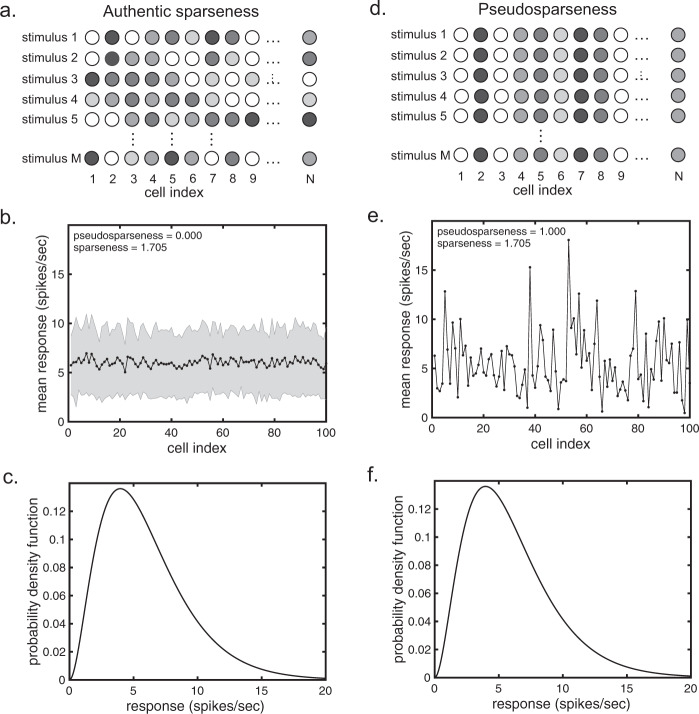
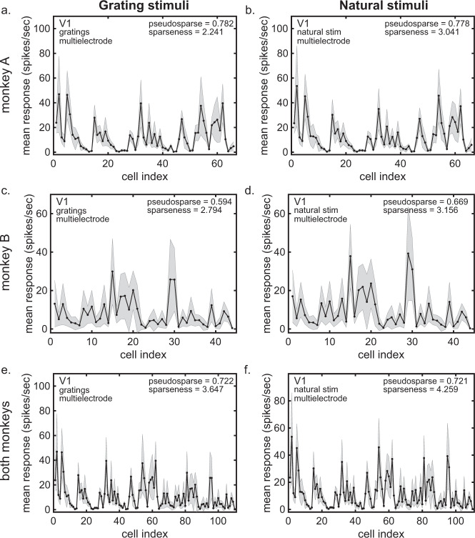
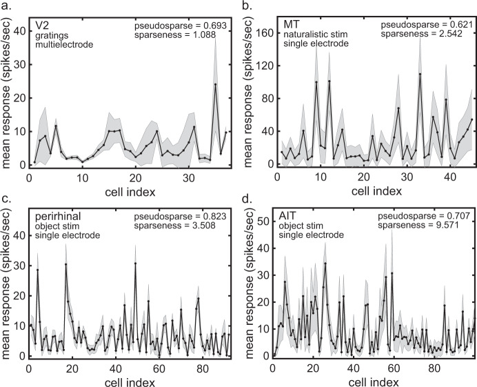
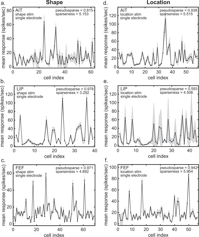
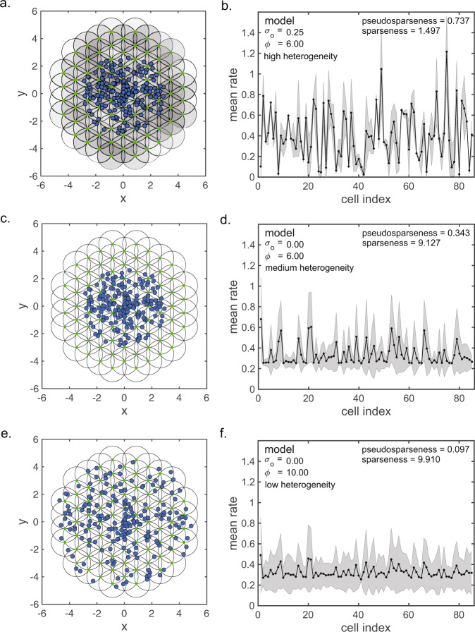
When measuring sparseness in neural populations as an indicator of efficient coding, an implicit assumption is that each stimulus activates a different random set of neurons. In other words, population responses to different stimuli are, on average, uncorrelated. Here we examine neurophysiological data from four lobes of macaque monkey cortex, including V1, V2, MT, anterior inferotemporal cortex, lateral intraparietal cortex, the frontal eye fields, and perirhinal cortex, to determine how correlated population responses are. We call the mean correlation the pseudosparseness index, because high pseudosparseness can mimic statistical properties of sparseness without being authentically sparse. In every data set we find high levels of pseudosparseness ranging from 0.59-0.98, substantially greater than the value of 0.00 for authentic sparseness. This was true for synthetic and natural stimuli, as well as for single-electrode and multielectrode data. A model indicates that a key variable producing high pseudosparseness is the standard deviation of spontaneous activity across the population. Consistently high values of pseudosparseness in the data demand reconsideration of the sparse coding literature as well as consideration of the degree to which authentic sparseness provides a useful framework for understanding neural coding in the cortex.

Fig. 1. Comparison between sparseness and pseudosparseness.

a–c Example showing authentic sparseness. a Responses of the same neural population to different stimuli, under authentic sparseness. Each row of circles shows the responses to a different stimulus, with gray levels indicating response levels. Population responses to different stimuli are uncorrelated and a different random set of neurons is activated by each stimulus. b An example population response spectrum for authentic sparseness. Mean stimulus response (black) and response standard deviation (gray shading) for each neuron in the population is plotted on the y-axis, with neurons assigned arbitrary index numbers along the x-axis. For this example, each stimulus produces a set of responses across the population described by a gamma distribution. Parameters for the gamma distribution are identical for each member of the stimulus set. The pseudosparseness index calculates the mean correlation coefficient between population response vectors between all members of the stimulus set. c Median probability density function (pdf) for the neural population responses for individual stimuli under authentic sparseness. Each stimulus produces a single pdf for the responses across the neural population, and then the median pdf from all stimuli is determined and shown. d–f Example showing pseudosparseness. d Responses of the same neural population to different stimuli, under pseudosparseness. Under pseudosparseness, population response vectors for different stimuli are correlated, so that the same set of neurons is always activated for all stimuli. e An example population response spectrum for pseudosparseness. The population spectrum is produced using the same gamma distribution for population responses as used for authentic sparseness. For pseudosparseness, however, population response vectors for different stimuli are perfectly correlated. Therefore, the population spectrum has a standard deviation of zero, and pseudosparseness = 1.0. f Median probability density function for individual stimulus responses under maximum pseudosparseness. Note that this probability density function is identical to that under authentic sparseness in c. In the plots for the model N = 100 neurons with n = 10,000 stimuli per neuron.

Fig. 2. Response spectra for V1, using multielectrodes with grating and natural stimuli.

a Monkey A response spectrum using grating stimuli. N = 66 neurons with n = 416 stimuli per neuron. b Monkey A response spectrum using natural stimuli. N = 66 neurons with n = 540 stimuli per neuron. c Monkey B response spectrum using grating stimuli. N = 44 neurons with n = 416 stimuli per neuron. d Monkey B response spectrum using natural stimuli. N = 44 neurons with n = 540 stimuli per neuron. e Pooled data from both monkeys using grating stimuli. f Pooled data from both monkeys using natural stimuli. Neurons were the same for each monkey when using grating or natural stimuli (Data from Coen-Cagli et al.). Mean pseudosparseness and median sparseness values (median because sparseness values are strongly right skewed) are given here and in subsequent figures. Gray error bars represent standard deviation.

Fig. 3. Response spectra for V1 using single-electrode data.

a Response spectrum using grating stimuli. N = 10 neurons with n = 416 stimuli per neuron. b Response spectrum using natural stimuli. N = 10 neurons with n = 540 stimuli per neuron. Neurons in a and b are the same. These single-electrode data were synthesized from multielectrode data (Data from Coen-Cagli et al.). c Response spectrum using synthetic stimuli. N = 24 neurons with 157 stimuli per neuron (Data from Lehky et al.^,). Gray error bars represent standard deviation.

Fig. 4. Comparison between multielectrode and single-electrode V1 data for pseudosparseness and sparseness values as a function of population size.

a Comparison of pseudosparseness using grating stimuli. b Comparison of pseudosparseness using natural stimuli. c Comparison of sparseness using grating stimuli. d Comparison of sparseness using natural stimuli. Single-electrode population was synthesized from multielectrode data by selecting one cell from different multielectrode recording sessions from the same data set. Multielectrode data was subsampled to produce various population sizes. Entire curves were generated for completeness, but the critical comparison is that between the N = 10 single-electrode population and the N = 10 multielectrode population. N = 5–60 neurons on the x-axis with 10,000 resampled population activities based on n = 416 stimuli (gratings) or n = 540 stimuli (natural images) for each neuron (Data from Coen-Cagli et al.).

Fig. 5. Response spectra for four extrastriate cortical areas using a variety of stimuli.

a Response spectrum from V2. N = 37 neurons with 8 stimuli per neuron (Data from Zandvakili and Kohn and Semedo et al.). b Response spectrum from MT. N = 45 neurons with 200 stimuli per neuron (Data from Nishimoto and Gallant). c Response spectrum from perirhinal cortex. N = 92 neurons with n = 110 stimuli per neuron (Data from Lehky and Tanaka). d Response spectrum from anterior inferotemporal cortex (AIT). N = 122 neurons with n = 110 stimuli per neuron (Data from Lehky and Tanaka). Gray error bars represent standard deviation.

Fig. 6. Response spectra for three cortical areas using either shape or retinotopic location stimuli.

a Anterior inferotemporal cortex (AIT) data for stimulus shape. N = 85 neurons with n = 8 stimuli per neuron (Data from Lehky and Sereno). b Lateral intraparietal cortex (LIP) data for stimulus shape. N = 53 neurons with n = 8 stimuli per neuron (Data from Lehky and Sereno). c Frontal eye field (FEF) data for stimulus shape. N = 72 neurons with n = 8 stimuli per neuron (Data from Peng et al.). d AIT data for stimulus location. N = 83 neurons with n = 8 stimuli per neuron (Data from Lehky et al. and Sereno and Lehky). e LIP data for stimulus location. N = 65 neurons with n = 8 stimuli per neuron (Data from Lehky et al. and Sereno and Lehky). f FEF data for stimulus location N = 62 neurons with n = 8 stimuli per neuron (Previously unpublished data). Gray error bars represent standard deviation.

Fig. 7. Model for generating various level of pseudosparseness in a population of receptive fields activated by random stimuli.

Top row: high pseudosparseness conditions. a Hexagonal grid of overlapping receptive fields in a 2D feature space (e.g., position, shape, etc.). Each receptive field has a Gaussian tuning curve in the feature space described in Eq. (2), with a small green dot indicating receptive field center and circle indicating receptive field drawn at space constant σ = 2 (in arbitrary units). Receptive spacing is η = 1.0 and receptive field dispersion (size of circular boundary of green dots) is γ = 10.0. Additional parameter values are gain mean μ_G = 1.0, gain standard deviation σ_G = 0.25, offset mean μ_O = 0.25, and offset standard deviation σ_O = 0.25. Blue dots indicate a random set of stimuli. Stimulus set dispersion (size of circular boundary of blue dots) is ϕ = 6. b Resulting response spectrum, showing high level of pseudosparseness = 0.737. Second and third rows: examples of two conditions producing lower pseudosparseness, namely, reducing the response offset level and increasing the stimulus set dispersion. These conditions make population responses less heterogeneous. c Receptive field mosaic with offset standard deviation reduced to σ_O = 0.0, indicated by receptive field gray levels being white. d Resulting response spectrum, showing a lower pseudosparseness compared to when response offset level is higher. e Receptive field mosaic with stimulus set dispersion increased to ϕ = 10, in addition to response offset again set to zero. f Increasing the stimulus set dispersion leads to further decrease in pseudosparseness. Gray error bars represent standard deviation.

References

1. Barlow, H. B. in Sensory Communication (ed. Rosenblith, W.) Ch. 13, 217–234 (MIT Press, 1961).
1. Simoncelli EP, Olshausen BA. Natural image statistics and neural representation. Annu. Rev. Neurosci. 2001;24:1193–1216. doi: 10.1146/annurev.neuro.24.1.1193. - DOI - PubMed
1. Olshausen BA, Field DJ. Sparse coding of sensory inputs. Curr. Opin. Neurobiol. 2004;14:481–487. doi: 10.1016/j.conb.2004.07.007. - DOI - PubMed
1. Földiák, P. In Handbook of Brain Theory and Neural Networks, 2nd edn (ed. Michael, A. Arbib) 1064–1068 (MIT Press, 2002).
1. Atick JJ. Could information theory provide an ecological theory of sensory processing? Network. 1992;3:213–251. doi: 10.1088/0954-898X_3_2_009. - DOI - PubMed
Publication types