Robust breast cancer detection in mammography and digital breast tomosynthesis using an annotation-efficient deep learning approach

Abstract

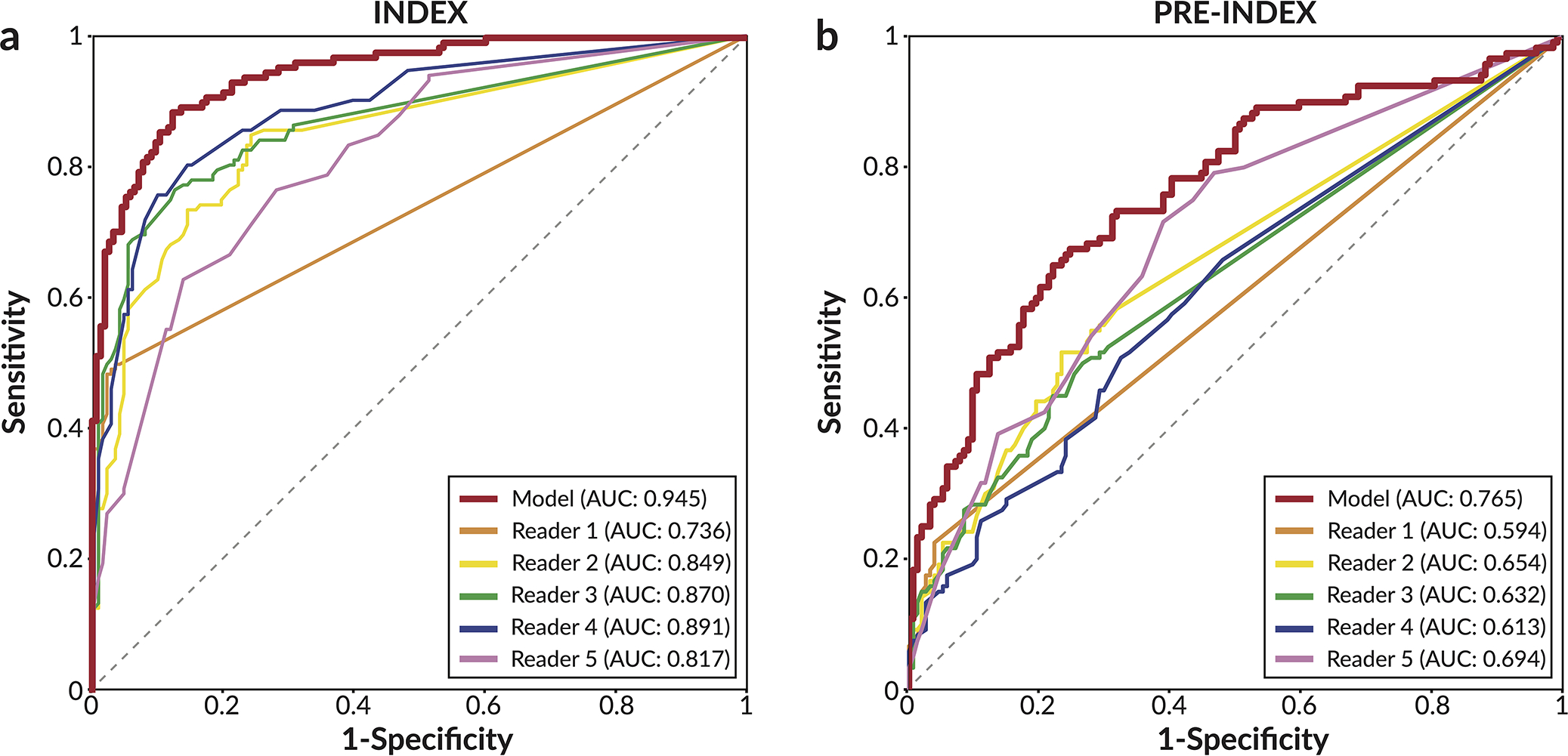
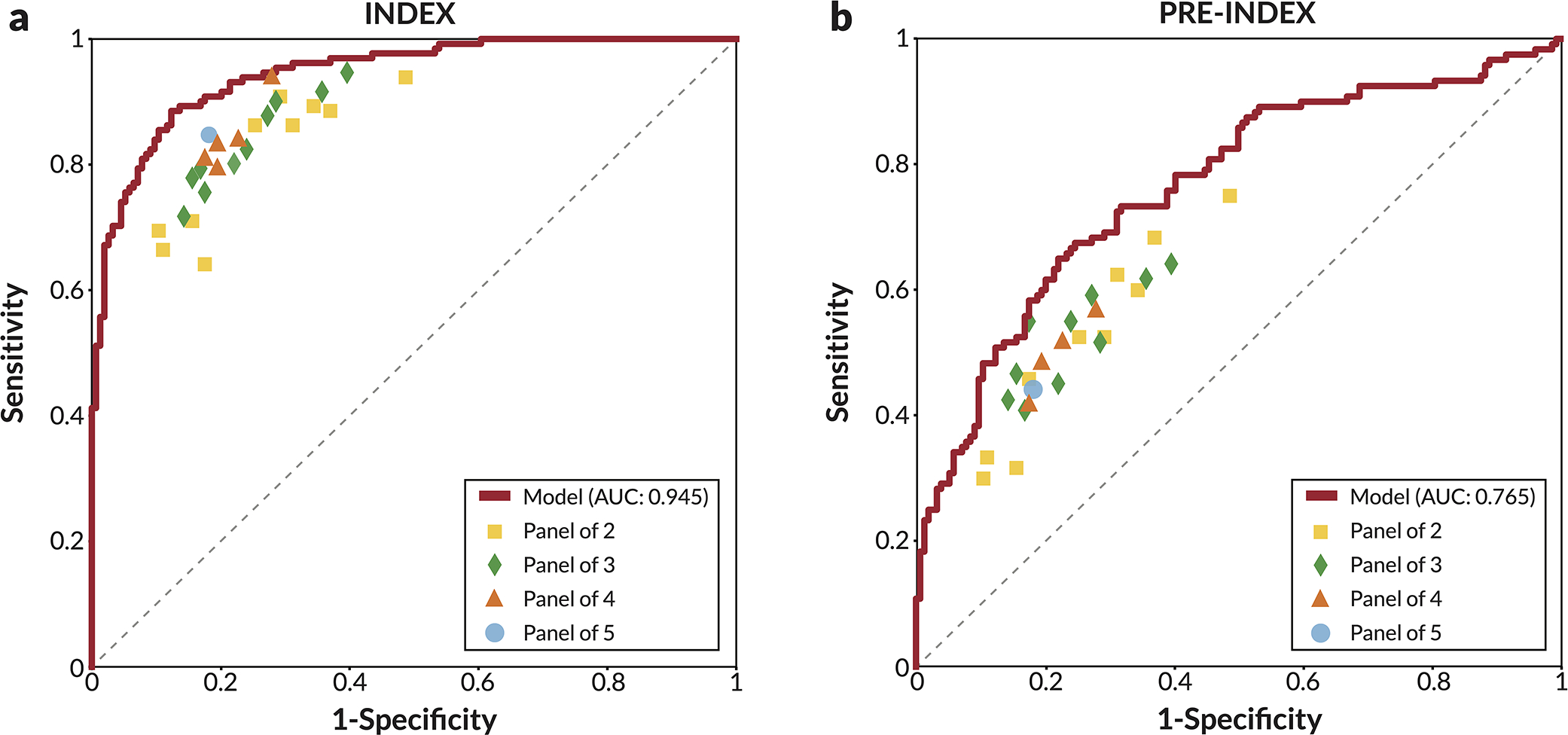
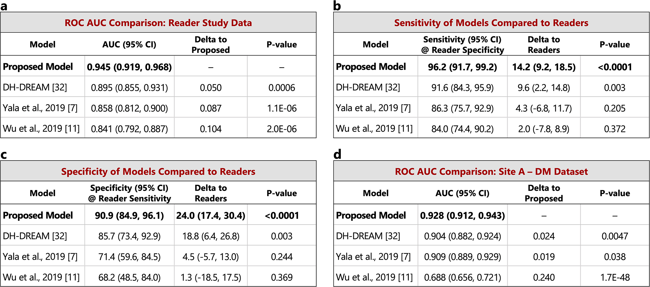
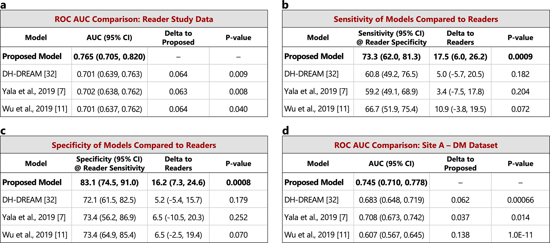
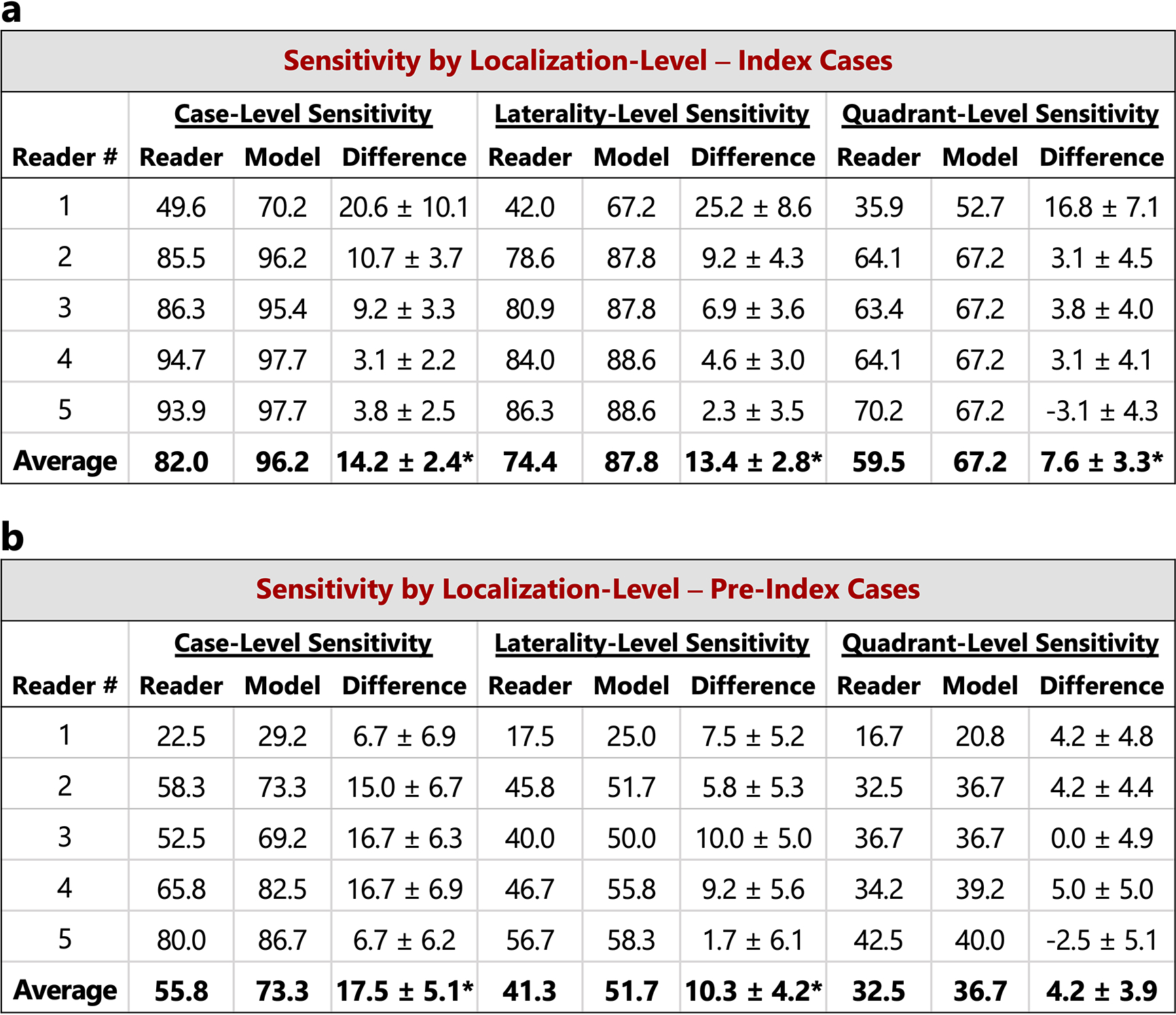
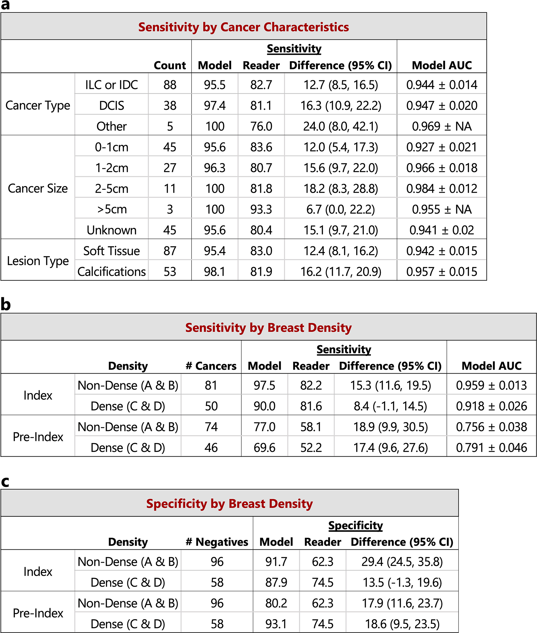
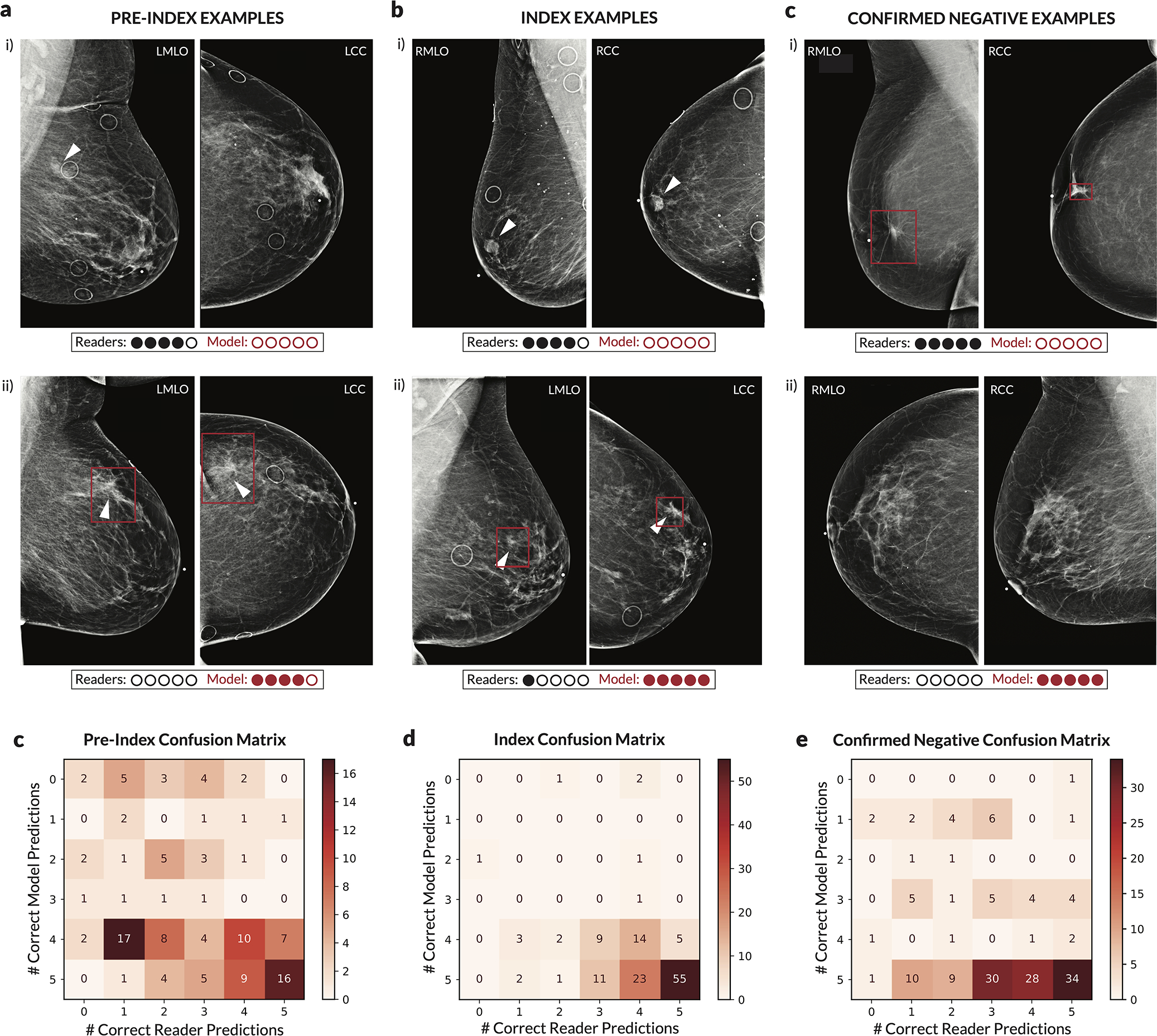
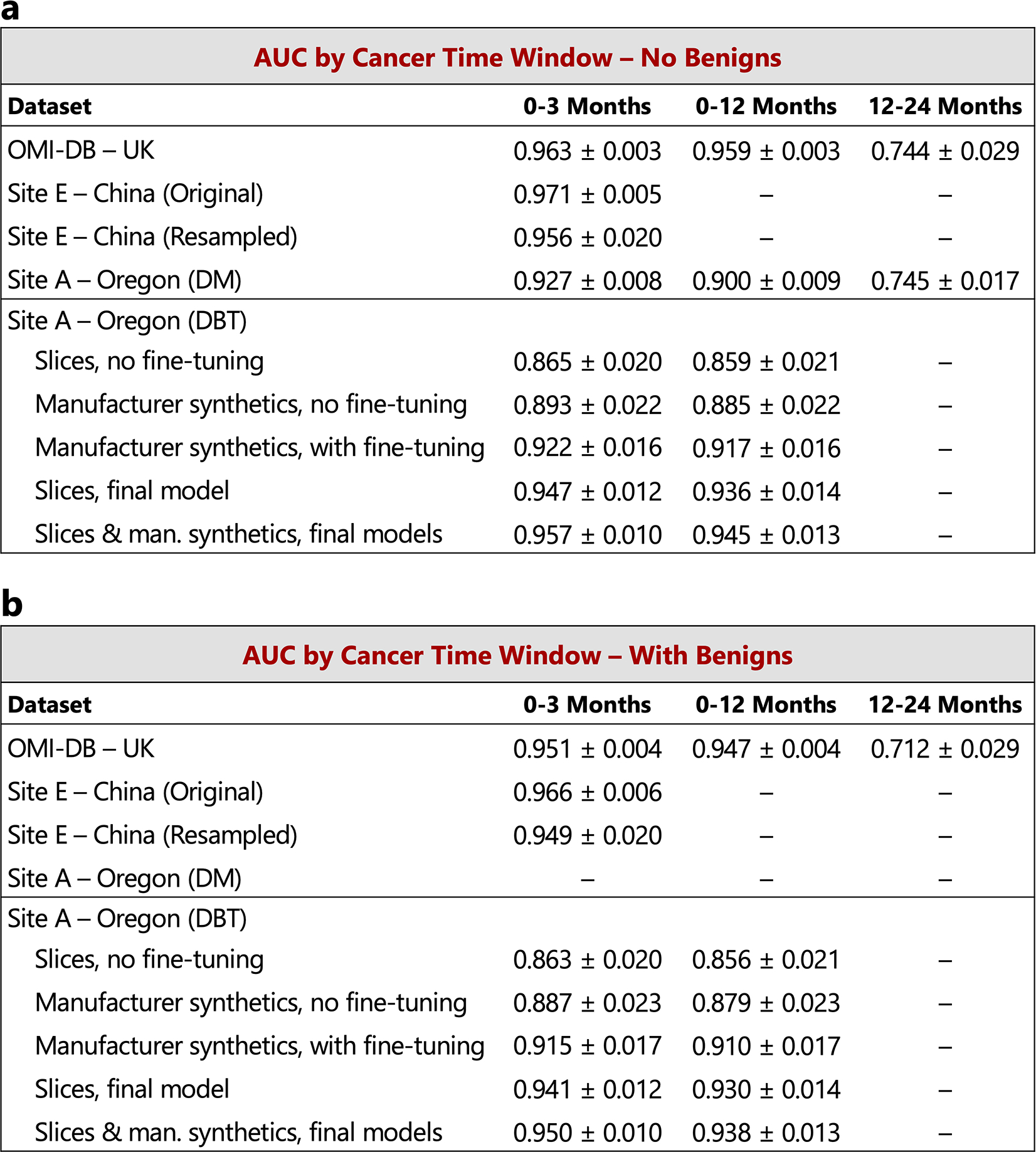
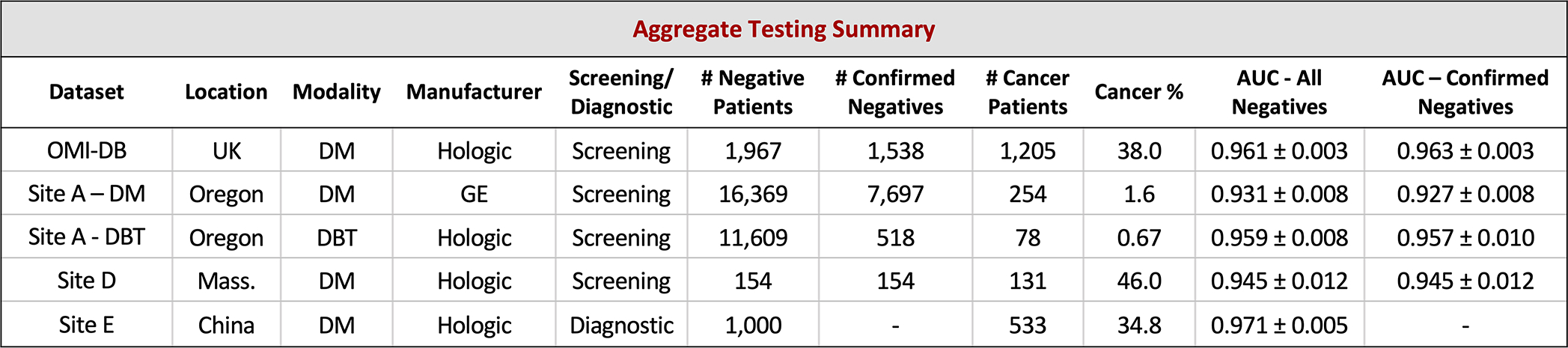
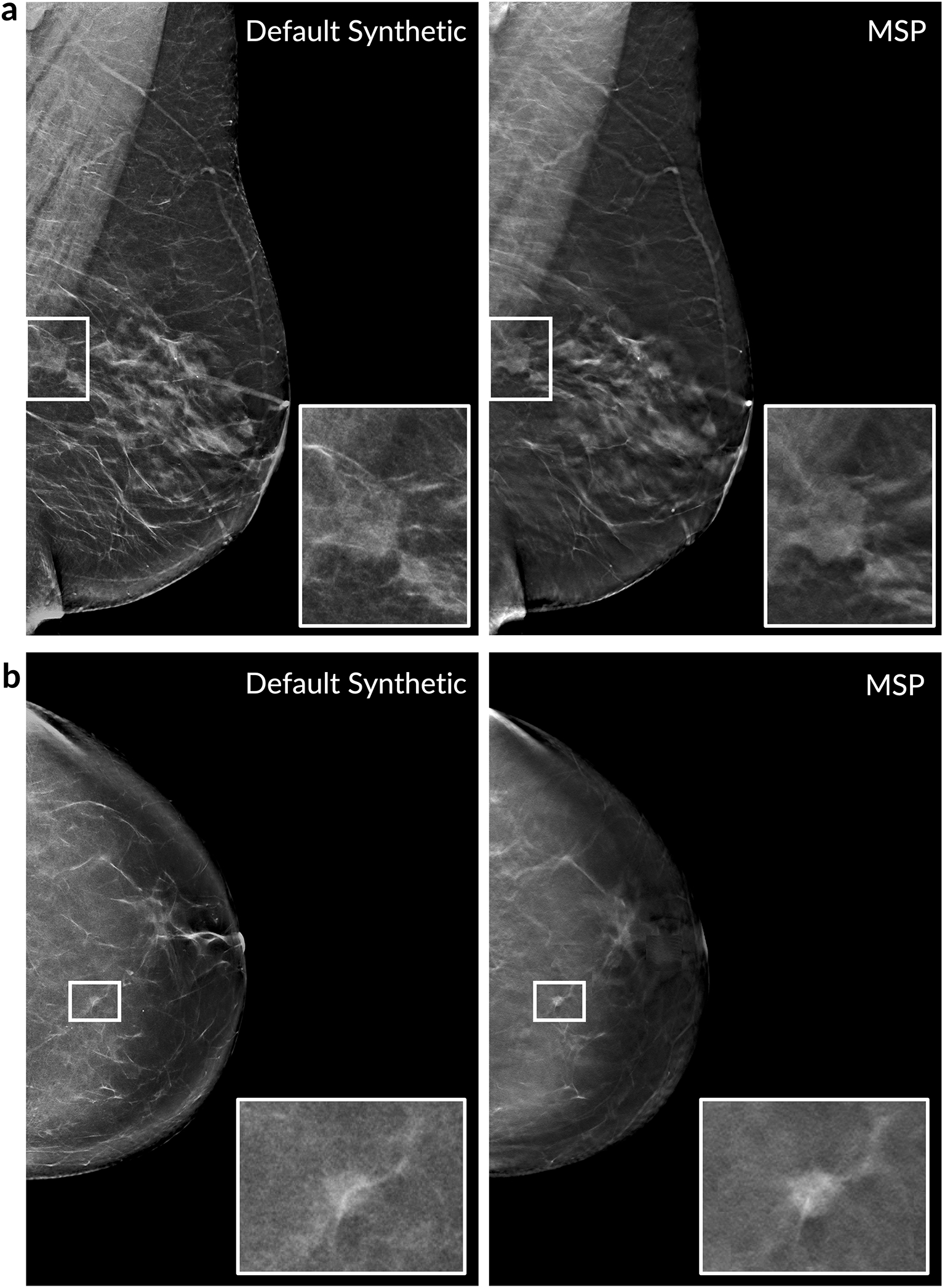
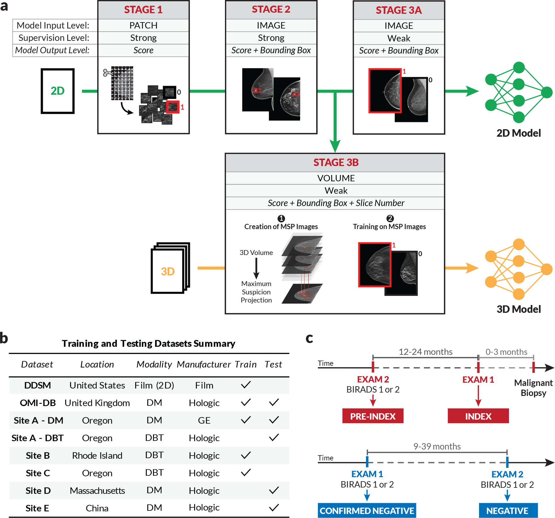
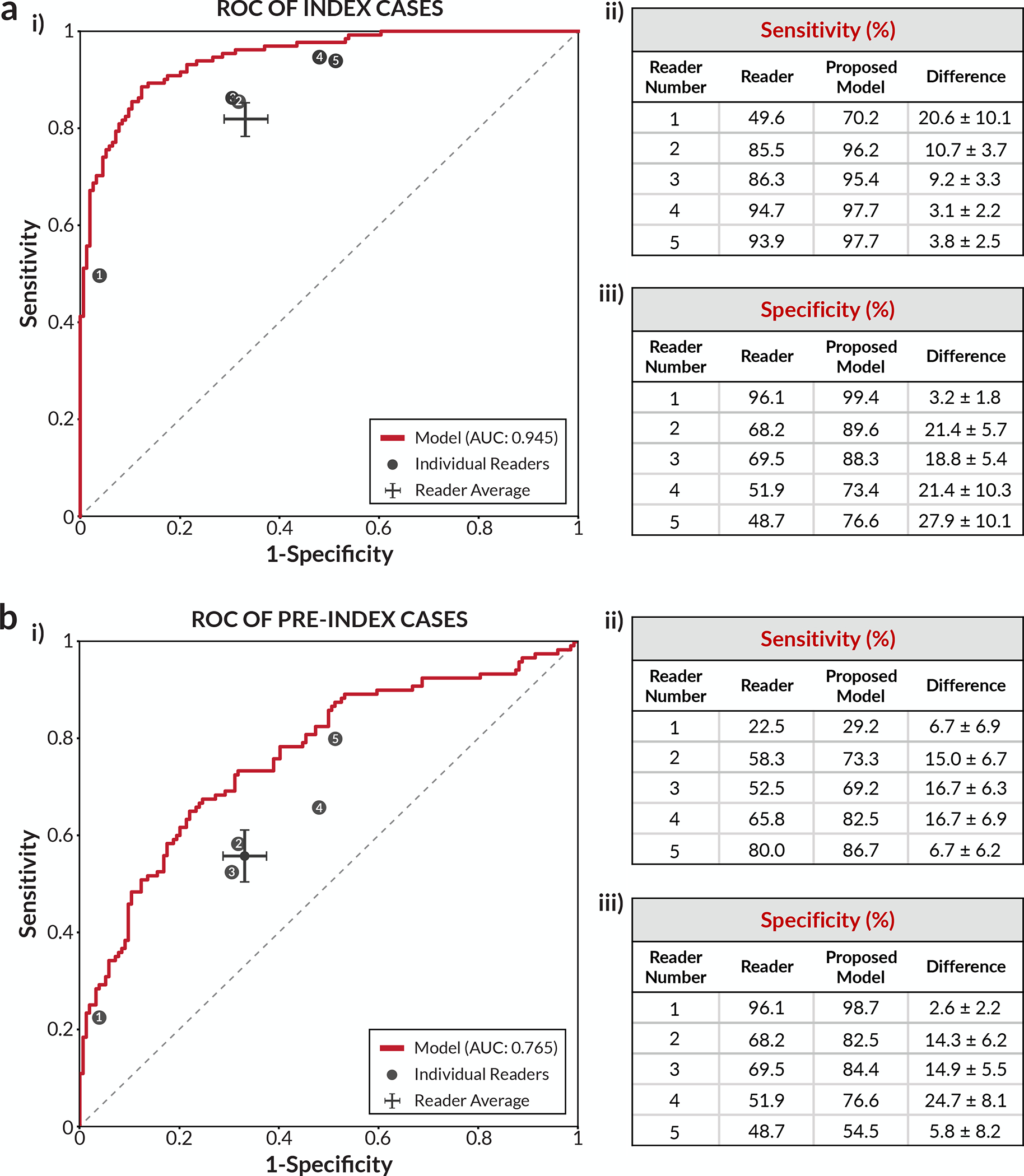
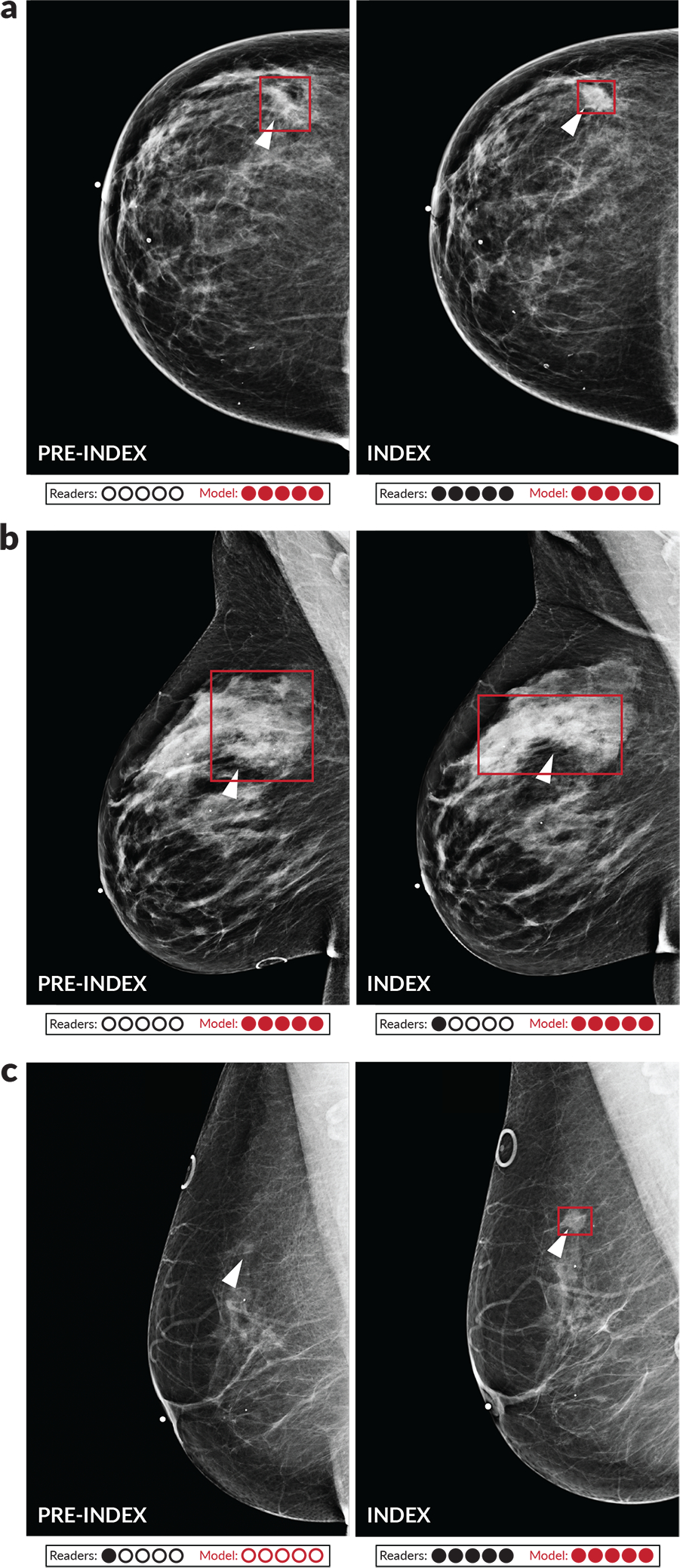
Breast cancer remains a global challenge, causing over 600,000 deaths in 2018 (ref. ¹). To achieve earlier cancer detection, health organizations worldwide recommend screening mammography, which is estimated to decrease breast cancer mortality by 20-40% (refs. ^2,3). Despite the clear value of screening mammography, significant false positive and false negative rates along with non-uniformities in expert reader availability leave opportunities for improving quality and access^4,5. To address these limitations, there has been much recent interest in applying deep learning to mammography^6-18, and these efforts have highlighted two key difficulties: obtaining large amounts of annotated training data and ensuring generalization across populations, acquisition equipment and modalities. Here we present an annotation-efficient deep learning approach that (1) achieves state-of-the-art performance in mammogram classification, (2) successfully extends to digital breast tomosynthesis (DBT; '3D mammography'), (3) detects cancers in clinically negative prior mammograms of patients with cancer, (4) generalizes well to a population with low screening rates and (5) outperforms five out of five full-time breast-imaging specialists with an average increase in sensitivity of 14%. By creating new 'maximum suspicion projection' (MSP) images from DBT data, our progressively trained, multiple-instance learning approach effectively trains on DBT exams using only breast-level labels while maintaining localization-based interpretability. Altogether, our results demonstrate promise towards software that can improve the accuracy of and access to screening mammography worldwide.

Extended Data Figure 1:. Reader ROC curves using Probability of Malignancy metric.

For each lesion deemed suspicious enough to warrant recall, readers assigned a 0–100 probability of malignancy (POM) score. Cases not recalled were assigned a score of 0. a) ROC curve using POM on the 131 index cancer cases and 154 confirmed negatives. In order of reader number, the reader AUCs are 0.736±0.023, 0.849±0.022, 0.870±0.021, 0.891±0.019, and 0.817±0.025. b) ROC curve using POM on the 120 pre-index cancer cases and 154 confirmed negatives. In order of reader number, the reader AUCs are 0.594±0.021, 0.654±0.031, 0.632±0.030, 0.613±0.033, and 0.694±0.031. The standard deviation for each AUC value was calculated via bootstrapping.

Extended Data Figure 2:. Results of model compared to synthesized panel of readers.

Comparison of model ROC curves to every combination of 2, 3, 4, and 5 readers. Readers were combined by averaging BIRADS scores, with sensitivity and specificity calculated using a threshold of 3. On both the (a) index cancer exams and (b) pre-index cancer exams, the model outperformed every combination of readers, as indicated by each combination falling below the model’s respective ROC curve. The reader study dataset consists of 131 index cancer exams, 120 pre-index cancer exams, and 154 confirmed negatives.

Extended Data Figure 3:. Comparison to recent work – index cancer exams.

The performance of the proposed model is compared to other recently published models on the set of index cancer exams and confirmed negatives from our reader study (a-c) and the “Site A - DM dataset” (d). P-values for AUC differences were calculated using the DeLong method [45] (two sided). Confidence intervals for AUC, sensitivity, and specificity were computed via bootstrapping. a) ROC AUC comparison: Reader study data (Site D). The Site D dataset contains 131 index cancer exams and 154 confirmed negatives. The DeLong method z-values corresponding to the AUC differences are, from top to bottom, 3.44, 4.87, and 4.76. b) Sensitivity of models compared to readers. Sensitivity was obtained at the point on the ROC curve corresponding to the average reader specificity. Delta values show the difference between model sensitivity and average reader sensitivity and the p-values correspond to this difference (computed via bootstrapping). c) Specificity of models compared to readers. Specificity was obtained at the point on the ROC curve corresponding to the average reader sensitivity. Delta values show the difference between model specificity and average reader specificity and the p-values correspond to this difference (computed via bootstrapping). d) ROC AUC comparison: Site A - DM dataset. Compared to the original dataset, 60 negatives (0.78% of the negatives) were excluded from the comparison analysis because at least one of the models were unable to successfully process these studies. All positives were successfully processed by all models, resulting in 254 index cancer exams and 7,637 confirmed negatives for comparison. The DeLong method z-values corresponding to the AUC differences are, from top to bottom, 2.83, 2.08, and 14.6.

Extended Data Figure 4:. Comparison to recent work – pre-index cancer exams.

The performance of the proposed model is compared to other recently published models on the set of pre-index cancer exams and confirmed negatives from our reader study (a-c) and the “Site A - DM dataset” (d). P-values for AUC differences were calculated using the DeLong method [45] (two sided). Confidence intervals for AUC, sensitivity, and specificity were computed via bootstrapping. a) ROC AUC comparison: Reader study data (Site D). The Site D dataset contains 120 pre-index cancer exams and 154 confirmed negatives. The DeLong method z-values corresponding to the AUC differences are, from top to bottom, 2.60, 2.66, and 2.06. b) Sensitivity of models compared to readers. Sensitivity was obtained at the point on the ROC curve corresponding to the average reader specificity. Delta values show the difference between model sensitivity and average reader sensitivity and the p-values correspond to this difference (computed via bootstrapping). c) Specificity of models compared to readers. Specificity was obtained at the point on the ROC curve corresponding to the average reader sensitivity. Delta values show the difference between model specificity and average reader specificity and the p-values correspond to this difference (computed via bootstrapping). d) ROC AUC comparison: Site A - DM dataset. Compared to the original dataset, 60 negatives (0.78% of the negatives) were excluded from the comparison analysis because at least one of the models were unable to successfully process these studies. All positives were successfully processed by all models, resulting in 217 pre-index cancer exams and 7,637 confirmed negatives for comparison. The DeLong method z-values corresponding to the AUC differences are, from top to bottom, 3.41, 2.47, and 6.81.

Extended Data Figure 5:. Localization-based sensitivity analysis.

In the main text, case-level results are reported. Here, we additionally consider lesion localization when computing sensitivity for the reader study. Localization-based sensitivity is computed at two levels - laterality and quadrant (see Methods). As in Figure 2 in the main text, we report the model’s sensitivity at each reader’s specificity (96.1, 68.2, 69.5, 51.9, and 48.7 for Readers 1–5 respectively) and at the reader average specificity (66.9). a) Localization-based sensitivity for the index cases (131 cases). b) Localization-based sensitivity for the pre-index cases (120 cases). For reference, the case-level sensitivities are also provided. We find that the model outperforms the reader average for both localization levels and for both index and pre-index cases (*p<0.05; Specific p-values: index- laterality: p<1e–4, index - quadrant: p=0.01, pre-index - laterality: p=0.01, pre-index - quadrant: p=0.14). The results in the tables below correspond to restricting localization to the top scoring predicted lesion for both reader and model (see Methods). If we allow localization by any predicted lesion for readers while still restricting the model to only one predicted bounding box, the difference between the model and reader average performance is as follows (positive values indicate higher performance by model): index - laterality: 11.2±2.8 (p=0.0001), index - quadrant: 4.7±3.3 (p=0.08), pre-index - laterality: 7.8±4.2 (p=0.04), pre-index - quadrant: 2.3±3.9 (p=0.28). P-values and standard deviations were computed via bootstrapping. Finally, we note that while the localization-based sensitivities of the model may seem relatively low on the pre-index cases, the model is evaluated in a strict scenario of only allowing one box per study and crucially, all of the pre-index effectively represent “misses” in the clinic. Even when set to a specificity of 90% [36], the model still detects a meaningful number of the missed cancers while requiring localization, with a sensitivity of 37% and 28% for laterality and quadrant localization, respectively.

Extended Data Figure 6:. Reader study case characteristics and performance breakdown.

The performance of the proposed deep learning model compared to the reader average grouped by various case characteristics is shown. For sensitivity calculations, the score threshold for the model is chosen to match the reader average specificity. For specificity calculations, the score threshold for the model is chosen to match the reader average sensitivity. a) Sensitivity and model AUC grouped by cancer characteristics, including cancer type, cancer size, and lesion type. The cases correspond to the index exams since the status of these features are unknown at the time of the pre-index exams. Lesion types are grouped by soft tissue lesions (masses, asymmetries, and architectural distortions) and calcifications. Malignancies containing lesions of both types are included in both categories (9 total cases). ‘NA’ entries for model AUC standard deviation indicate that there were too few positive samples for bootstrap estimates. The 154 confirmed negatives in the reader study dataset were used for each AUC calculation. b) Sensitivity and model AUC by breast density. The breast density is obtained from the original radiology report for each case. c) Specificity by breast density. Confidence intervals and standard deviations were computed via bootstrapping.

Extended Data Figure 7:. Discrepancies between readers and deep learning model.

For each case, the number of readers that correctly classified the case was calculated along with the number of times the deep learning model would classify the case correctly when setting a score threshold to correspond to either the specificity of each reader (for index and pre-index cases) or the sensitivity of each reader (for confirmed negative cases). Thus, for each case, 0–5 readers could be correct, and the model could achieve 0–5 correct predictions. The evaluation of the model at each of the operating points dictated by each reader was done to ensure a fair, controlled comparison (i.e., when analyzing sensitivity, specificity is controlled). We note that in practice a different operating point (i.e., score threshold) may be used. The examples shown illustrate discrepancies between model and human performance, with the row of dots below each case illustrating the number of correct predictions. Red boxes on the images indicate the model’s bounding box output. White arrows indicate the location of a malignant lesion. a) Examples of pre-index cases where the readers outperformed the model (i) and where the model outperformed the readers (ii). b) Examples of index cases where the readers outperformed the model (i) and where the model outperformed the readers (ii). c) Examples of confirmed negative cases where the readers outperformed the model (i) and where the model outperformed the readers (ii). For the example in c.i.), the patient previously had surgery six years ago for breast cancer at the location indicated by the model, but the displayed exam and the subsequent exam the following year were interpreted as BIRADS 2. For the example in c.ii.), there are posterior calcifications that had previously been biopsied with benign results, and all subsequent exams (including the one displayed) were interpreted as BIRADS 2. d) Full confusion matrix between the model and readers for pre-index cases. e) Full confusion matrix between the model and readers for index cases. f) Full confusion matrix between the model and readers for confirmed negative cases.

Extended Data Figure 8:. Performance of proposed models under different case compositions.

Unless otherwise noted, in the main text we chose case compositions and definitions to match those of the reader study, specifically index cancer exams were mammograms acquired within 3 months preceding a cancer diagnosis and non-cancers were negative mammograms (BIRADS 1 or 2) that were “confirmed” by a subsequent negative screen. Here, we additionally consider (a) a 12-month definition of index cancers, i.e., mammograms acquired within 0–12 months preceding a cancer diagnosis, as well as (b) including biopsy-proven benign cases as non-cancers. The 3-month time window for cancer diagnosis includes 1,205, 533, 254, and 78 cancer cases for OMI-DB, Site E, Site A - DM, and Site A - DBT, respectively. The number of additional cancer cases included in the 12-month time window is 38, 46, and 7 for OMI-DB, Site A - DM, and Site A - DBT, respectively. A 12–24 month time window results in 68 cancer cases for OMI-DB and 217 cancer cases for Site A - DM. When including benign cases, those in which the patient was recalled and ultimately biopsied with benign results, we use a 10:1 negative to benign ratio to correspond with a typical recall rate in the United States [36]. For a given dataset, the negative cases are shared amongst all cancer time window calculations, with 1,538, 1,000, 7,697, and 518 negative cases for OMI-DB, Site E, Site A - DM, and Site A - DBT, respectively. For all datasets except Site E, the calculations below involve confirmed negatives. Dashes indicate calculations that are not possible given the data and information available for each site. The standard deviation for each AUC value was calculated via bootstrapping.

Extended Data Figure 9:. Aggregate summary of testing data and results.

Results are calculated using index cancer exams and both confirmed negatives and all negatives (confirmed and unconfirmed) separately. While requiring negative confirmation excludes some data, similar levels of performance are observed across both confirmation statuses in each dataset. Across datasets, performance is also relatively consistent, though there is some variation as might be expected given different screening paradigms and population characteristics. Further understanding of performance characteristics across these populations and other large-scale cohorts will be important future work. The standard deviation for each AUC value was calculated via bootstrapping.

Extended Data Figure 10:. Examples of maximum suspicion projection (MSP) images.

Two cancer cases are presented. Left column: Default 2D synthetic images. Right column: MSP images. The insets highlight the malignant lesion. In both cases, the deep learning algorithm scored the MSP image higher for the likelihood of cancer (a: 0.77 vs. 0.14, b: 0.87 vs. 0.31). We note that the deep learning algorithm correctly localized the lesion in both of the MSP images as well.

Figure 1:. Model training approach and data summary.

a) To effectively leverage both strongly and weakly-labeled data while mitigating overfitting, we progressively train our deep learning models in a series of stages. Stage 1 consists of patch-level classification using cropped image patches from 2D mammograms [15]. In Stage 2, the model trained in Stage 1 is used to initialize the feature backbone of a detection-based model. The detection model, which outputs bounding boxes with corresponding classification scores, is then trained end-to-end in a strongly-supervised manner on full images. Stage 3 consists of weakly-supervised training, for both 2D and 3D mammography. For 2D (Stage 3a), the detection network is trained for binary classification in an end-to-end, multiple-instance learning fashion where an image-level score is computed as a maximum over bounding box scores. For 3D (Stage 3b), the model from Stage 2 is used to condense each DBT stack into an optimized 2D projection by evaluating the DBT slices and extracting the most suspicious regions of interest at each x-y spatial location. The model is then trained on these “maximum suspicion projection” (MSP) images using the approach in Stage 3a. b) Summary of training and testing datasets. c) Illustration of exam definitions used here.

Figure 2:. Reader study results.

a) Index cancer exams & confirmed negatives. i) The proposed deep learning model outperformed all five radiologists on the set of 131 index cancer exams and 154 confirmed negatives. Each data point represents a single reader, and the ROC curve represents the performance of the deep learning model. The cross corresponds to the mean radiologist performance with the lengths of the cross indicating 95% confidence intervals. ii) Sensitivity of each reader and the corresponding sensitivity of the proposed model at a specificity chosen to match each reader. iii) Specificity of each reader and the corresponding specificity of the proposed model at a sensitivity chosen to match each reader. b) Pre-index cancer exams & confirmed negatives. i) The proposed deep learning model also outperformed all five radiologists on the early detection task. The dataset consisted of 120 pre-index cancer exams - which are defined as mammograms interpreted as negative 12–24 months prior to the index exam in which cancer was found - and 154 confirmed negatives. The cross corresponds to the mean radiologist performance with the lengths of the cross indicating 95% confidence intervals. ii) Sensitivity of each reader and the corresponding sensitivity of the proposed model at a specificity chosen to match each reader. iii) Specificity of each reader and the corresponding specificity of the proposed model at a sensitivity chosen to match each reader. For the sensitivity and specificity tables, the standard deviation of the model minus reader difference was calculated via bootstrapping.

Figure 3:. Examples of index and pre-index cancer exam pairs.

Images from three patients with biopsy-proven malignancies are displayed. For each patient, an image from the index exam from which the cancer was discovered is shown on the right, and an image from the prior screening exam acquired 12–24 months earlier and interpreted as negative is shown on the left. From top to bottom, the number of days between the index and pre-index exams is 378, 629, and 414. The dots below each image indicate reader and model performance. Specifically, the number of infilled black dots represent how many of the five readers correctly classified the corresponding case and the number of infilled red dots represent how many times the model would correctly classify the case if the model score threshold was individually set to match the specificity of each reader. The model is thus evaluated at five binary decision thresholds for comparison purposes, and we note that a different binary score threshold may be used in practice. Red boxes on the images indicate the model’s bounding box output. White arrows indicate the location of the malignant lesion. a) A cancer that was correctly classified by all readers and the deep learning model at all thresholds in the index case, but only detected by the model in the pre-index case. b) A cancer that was detected by the model in both the pre-index and index case, but only detected by one reader in the index case and zero readers in the pre-index case. c) A cancer that was detected by the readers and the model in the index case, but only detected by one reader in the pre-index case. The absence of a red bounding box indicates that the model did not detect the cancer.

References

1. Bray F, Ferlay J, Soerjomataram I, Siegel RL, Torre LA, and Jemal A Global cancer statistics 2018: GLOBOCAN estimates of incidence and mortality worldwide for 36 cancers in 185 countries. CA: A Cancer Journal for Clinicians 68(6), 394–424 (2018). - PubMed
1. Berry DA, Cronin KA, Plevritis SK, Fryback DG, Clarke L, Zelen M, Mandelblatt JS, Yakovlev AY, Habbema JDF, and Feuer EJ Effect of screening and adjuvant therapy on mortality from breast cancer. New England Journal of Medicine 353(17), 1784–1792 (2005). - PubMed
1. Seely JM and Alhassan T Screening for breast cancer in 2018 - what should we be doing today?. Current oncology (Toronto, Ont.) 25(Suppl 1), S115–S124 6 (2018). - PMC - PubMed
1. Majid AS, Shaw De Paredes E, Doherty RD, Sharma NR, and Salvador X Missed breast carcinoma: pitfalls and pearls. RadioGraphics 23, 881–895 (2003). - PubMed
1. Rosenberg RD, Yankaskas BC, Abraham LA, Sickles EA, Lehman CD, Geller BM, Carney PA, Kerlikowske K, Buist DS, Weaver DL, Barlow WE, and Ballard-Barbash R Performance benchmarks for screening mammography. Radiology 241(1), 55–66 (2006). - PubMed
METHODS-ONLY REFERENCES
1. Otsu N A Threshold Selection Method from Gray-Level Histograms. IEEE Transactions on Systems, Man, and Cybernetics 9(1), 62–66 (1979).
1. He K, Zhang X, Ren S, and Sun J Deep Residual Learning for Image Recognition. In The IEEE Conference on Computer Vision and Pattern Recognition (CVPR), 770–778, (2016).
1. Kingma DP and Ba J Adam: a method for stochastic optimization. In The 3rd International Conference on Learning Representations (ICLR) (2015).
1. Lin T, Goyal P, Girshick R, He K, and Dollár P Focal loss for dense object detection. In The IEEE International Conference on Computer Vision (ICCV), 2999–3007, (2017).
1. Gallas BD, Chen W, Cole E, Ochs R, Petrick N, Pisano ED, Sahiner B, Samuelson FW, and Myers K Impact of prevalence and case distribution in lab-based diagnostic imaging studies. Journal of Medical Imaging 6(01), 1 1 (2019). - PMC - PubMed
Publication types