Streamlining data-intensive biology with workflow systems

Abstract

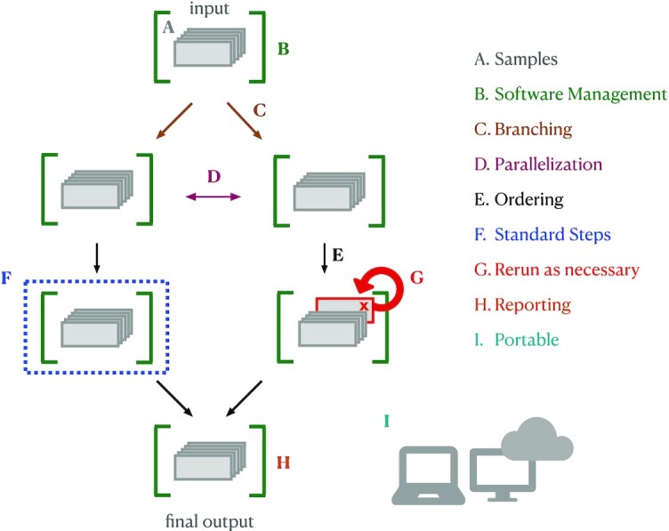
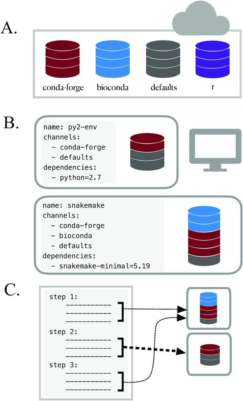
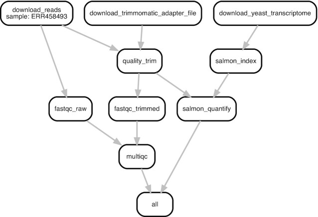
As the scale of biological data generation has increased, the bottleneck of research has shifted from data generation to analysis. Researchers commonly need to build computational workflows that include multiple analytic tools and require incremental development as experimental insights demand tool and parameter modifications. These workflows can produce hundreds to thousands of intermediate files and results that must be integrated for biological insight. Data-centric workflow systems that internally manage computational resources, software, and conditional execution of analysis steps are reshaping the landscape of biological data analysis and empowering researchers to conduct reproducible analyses at scale. Adoption of these tools can facilitate and expedite robust data analysis, but knowledge of these techniques is still lacking. Here, we provide a series of strategies for leveraging workflow systems with structured project, data, and resource management to streamline large-scale biological analysis. We present these practices in the context of high-throughput sequencing data analysis, but the principles are broadly applicable to biologists working beyond this field.

Keywords: automation; data-intensive biology; repeatability; workflows.

Figure 1:

Workflow systems: bioinformatics workflow systems have built-in functionality that facilitates and simplifies running analysis pipelines. A. Samples: workflow systems enable the user to use the same code to run each step on each sample. Samples can be easily added if the analysis expands. B. Software management: integration with software management tools (e.g., conda, singularity, docker) can automate software installation for each step. C. Branching, D. parallelization, and E. ordering: workflow systems handle conditional execution, ensuring that tasks are executed in the correct order for each sample file, including executing independent steps in parallel if possible given the resources provided. F. Standard steps: many steps are now considered “standard” (e.g., quality control). Workflow languages keep all information for a step together and can be written to enable remixing and reuse of individual steps across pipelines. G. Rerun as necessary: workflow systems keep track of which steps executed properly and on which samples, and allow failed steps (or additional steps) to be rerun rather than re-executing the entire workflow. H. Reporting: workflow languages enable comprehensive reporting on workflow execution and resource utilization by each tool. I. Portability: analyses written in workflow languages (with integrated software management) can be run across computing systems without changes to code.

Figure 2:

The conda package and environment manager simplifies software installation and management. A. Conda recipe repositories: each program distributed via conda has a “recipe” describing all software dependencies needed for installation using conda (each of which must also be installable via conda). Recipes are stored and managed in the cloud in separate “channels,” some of which specialize in particular fields or languages (e.g., the “bioconda” channel specializes in bioinformatics software, while the “conda-forge” channel is a more general effort to provide and maintain standardized conda packages for a wide range of software) [11]. B. Use conda environments to avoid installation conflicts: conda does not require root privileges for software installation, thus enabling use by researchers working on shared cluster systems. However, even user-based software installation can encounter dependency conflicts. For example, you might need to use Python2 to install and run a program (e.g., older scripts written by members of your laboratory), while also using snakemake to execute your workflows (requires Python ≥3.5). By installing each program into an isolated “environment” that contains only the software required to run that program, you can ensure that all programs used throughout your analysis will run without issue. Using small, separate environments for your software, specifying the desired software version, and building many simple environments to accommodate different steps in your workflow is critical for reducing the amount of time it takes conda to resolve dependency conflicts between different software tools (“solve” an environment). Conda virtual environments can be created and installed either on the command line or via an environment YAML file, as shown. In this case, the environment file also specifies which conda channels to search and download programs from. When specified in a YAML file, conda environments are easily transferable between computers and operating systems. C. Most workflow management software enables specification of individual software environments for each step. In this example, steps 1 and 3 rely on the same environment, while step 2 uses a different environment. Broad community adoption has resulted in a proliferation of both conda-installable scientific software and tools that leverage conda installation specifications. For example, the Mamba package manager is an open source reimplementation of the conda manager that can install conda-style environments with increased efficiency [51]. The BioContainers Registry is a project that automatically builds and distributes docker and singularity containers for bioinformatics software packages using each package's conda installation recipe [52].

Figure 3:

Consistent and informative file naming improves organization and interpretability. For ease of grouping and referring to input files, it is useful to keep unique sample identification in the filename, often with a metadata file explaining the meaning of each unique descriptor. For analysis scripts, it can help to implement a numbering scheme, where the name of the first file in the analysis begins with “00,” the next with “01,” and so on. For output files, it can help to add a short, unique identifier to output files processed with each analysis step. This particular file is a RAD-seq fastq file of a fish species that has been preprocessed with a fastq quality trimming tool.

Figure 4:

Examples of computational notebooks. Computational notebooks allow the user to mix text, code, and results in 1 document. A. RMarkdown document viewed in the RStudio integrated development environment; B. rendered HTML file produced by knitting the RMarkdown document [55]. C. Jupyter Notebook, where code, text, and results are rendered inline as each code chunk is executed [56]. The second grey chunk is a raw Markdown chunk with text that will be rendered inline when executed. Both notebooks generate a histogram of a metadata feature, number of generations, from a long-term evolution experiment with Escherichia coli [57]. Computational notebooks facilitate sharing by packaging narrative, code, and visualizations together. Sharing can be enhanced further by packaging computational notebooks with tools like Binder [58]. Binder builds an executable environment (capable of running RStudio and jupyter notebooks) out of a GitHub repository using package management systems and docker to build reproducible and executable software environments as specified in the repository. Binders can be shared with collaborators (or students in a classroom setting), and analysis and visualization can be ephemerally reproduced or altered from the code provided in computational notebooks.

Figure 5:

A directed acyclic graph (DAG) that illustrates connections between all steps of a sequencing data analysis workflow. Each box represents a step in the workflow, while lines connect sequential steps. The DAG shown in this figure illustrates a real bioinformatics workflow for RNA-seq quantification that was generated by modifying the default Snakemake workflow DAG. This example of an initial workflow used only to quality control and then quantify 1 FASTQ file against a transcriptome more than doubles the amount of files in a project. When the number of steps are expanded to carry out a full research analysis and the number of initial input files are increased, a workflow can generate hundreds to thousands of intermediate files. Fortunately, workflow system coordination alleviates the need for a user to directly manage file interdependencies. For a larger analysis DAG, see [60].

Figure 6:

Version control systems (e.g., Git, Mercurial) work by storing incremental differences in files from 1 saved version (“commit”) to the next. To visualize the differences between each version, text editors such as Atom and online services such as GitHub, GitLab, and Bitbucket use red highlighting to denote deletions and green highlighting to denote additions. In this trivial example, a typographical error in version 1 (in pink) was corrected in version 2 (in green). These systems are extremely useful for code and manuscript development because it is possible to return to the snapshot of any saved version. This means that version control systems save you from accidental deletions, preserve code that you thought you no longer needed, and preserve a record of project changes over time.

Figure 7:

Interactive visualizations facilitate sharing and repeatability. A. Interactive visualization dashboard in the Pavian Shiny app for metagenomic analysis [64, 65]. Shiny allows you to build interactive web pages using R code. Data are manipulated by R code in real time in a web page, producing analysis and visualizations of a dataset. Shiny apps can contain user-specifiable parameters, allowing a user to control visualizations or analyses. In (A), sample PT1 is selected, and taxonomic ranks class and order are excluded. Shiny apps allow collaborators who may or may not know R to modify R visualizations to fit their interests. B. Plotly heat map of transcriptional profiling in human brain samples [66]. Hovering over a cell in the heat map displays the sample names from the x and y axis, as well as the intensity value. Plotting tools such as plotly and vega-lite produce single interactive plots that can be shared with collaborators or integrated into websites [67, 68]. Interactive visualizations are also helpful in exploratory data analysis.

Figure 8:

Use Checksums to ensure file integrity. Checksum programs (e.g., md5, sha256) encode file size and content in a single value known as a “checksum.” For any given file, this value will be identical across platforms when calculated using the same checksum program. When transferring files, calculate the value of the checksum prior to transfer, and then again after transfer. If the value is not identical, there was an error introduced during transfer (e.g., file truncation). Checksums are often provided alongside publicly available files so that you can verify proper download. Tools like rsync and rclone that automate file transfers use checksums internally to verify that files were transferred properly, and some GUI file transfer tools (e.g., Cyberduck [109]) can assess checksums when they are provided [107]. If you generated your own data and receieved sequencing files from a sequencing center, be certain that you also receive a checksum for each of your files to ensure that they download properly.

Figure 9:

Visualizations produced by MultiQC. MultiQC finds and automatically parses log files from other tools and generates a combined report and parsed data tables that include all samples. MultiQC currently supports 88 tools. A. MultiQC summary of FastQC Per Sequence GC Content for 1,905 metagenome samples. FastQC provides quality control measurements and visualizations for raw sequencing data from a single sample and is a near-universal first step in sequencing data analysis because of the insights that it provides [110, 111]. FastQC measures and summarizes 10 quality metrics and provides recommendations for whether an individual sample is within an acceptable quality range. Not all metrics readily apply to all sequencing data types. For example, while multiple GC peaks might be concerning in whole-genome sequencing of a bacterial isolate, we would expect a non-normal distribution for some metagenome samples that contain organisms with diverse GC content. Samples like this can be seen in red in this figure. B. MultiQC summary of Salmon quant reads mapped per sample for RNA-seq samples [112]. In this figure, we see that MultiQC summarizes the number of reads mapped and percent of reads mapped, 2 values that are reported in the Salmon log files.

References

1. Ewels PA, Peltzer A, Fillinger S, et al. The nf-core framework for community-curated bioinformatics pipelines. Nat Biotechnol. 2020;38(3):276–8. - PubMed
1. Barone L, Williams J, Micklos D. Unmet needs for analyzing biological big data: A survey of 704 NSF principal investigators. PLoS Comput Biol. 2017;13(10):e1005755. - PMC - PubMed
1. Grüning B, Chilton J, Köster J, et al. Practical computational reproducibility in the life sciences. Cell Syst. 2018;6(6):631–5. - PMC - PubMed
1. Atkinson M, Gesing S, Montagnat J, et al. Scientific workflows: Past, present and future. Future Gener Comput Syst. 2017;75:216–27.
1. Conery JS, Catchen JM, Lynch M. Rule-based workflow management for bioinformatics. VLDB J. 2005;14:318–29.
Publication types