Greenhouse conditions in lower Eocene coastal wetlands?-Lessons from Schöningen, Northern Germany

Abstract

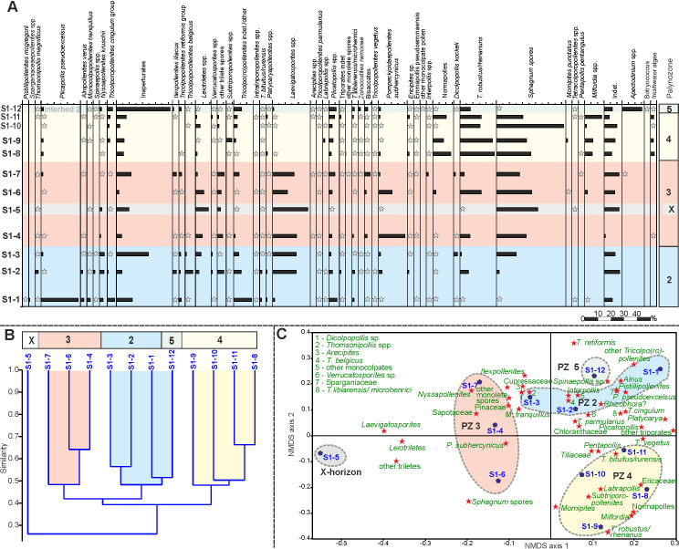
The Paleogene succession of the Helmstedt Lignite Mining District in Northern Germany includes coastal peat mire records from the latest Paleocene to the middle Eocene at the southern edge of the Proto-North Sea. Therefore, it covers the different long- and short-term climate perturbations of the Paleogene greenhouse. 56 samples from three individual sections of a lower Eocene seam in the record capture the typical succession of the vegetation in a coastal wetland during a period that was not affected by climate perturbation. This allows facies-dependent vegetational changes to be distinguished from those that were climate induced. Cluster analyses and NMDS of well-preserved palynomorph assemblages reveal four successional stages in the vegetation during peat accumulation: (1) a coastal vegetation, (2) an initial mire, (3) a transitional mire, and (4) a terminal mire. Biodiversity measures show that plant diversity decreased significantly in the successive stages. The highly diverse vegetation at the coast and in the adjacent initial mire was replaced by low diversity communities adapted to wet acidic environments and nutrient deficiency. The palynomorph assemblages are dominated by elements such as Alnus (Betulaceae) or Sphagnum (Sphagnaceae). Typical tropical elements which are characteristic for the middle Eocene part of the succession are missing. This indicates that a more warm-temperate climate prevailed in northwestern Germany during the early lower Eocene.

Fig 1. Paleogeographic map of Northwestern Europe during the lower Eocene.

The map shows the Helmstedt Embayment at the southern edge of the Proto-North Sea (H) in relation to important middle Eocene fossil localities in Germany, such as the Geiseltal (G), Messel (M), and Eckfeld (E); adapted from [34, 40].

Fig 2. The regional setting of the Helmstedt Lignite Mining District.

(A) Geologic structural map of the area between the major uplifts of the actual Harz Mountains to the South and the Flechtingen Rise in the north (modified after [36]). The salt pillows and diapirs are not exposed at the surface, but buried under Mesozoic and Cenozoic sedimentary rocks. The red frame marks the detail presented in (C) (B = Braunschweig, H = Helmstedt, S = Schöningen, E = Egeln, St = Staßfurt). (B) Cross-section through the study area, showing the Helmstedt-Staßfurt salt wall and related synclines (modified after [36]). (C) The former opencast mines Schöningen Nordfeld and Schöningen Südfeld east of Schöningen. The positions of the three studied sections of Seam 1 are indicated. The map has been rendered with the software Maperitive using geodata from OpenStreetMap.

Fig 3. Stratigraphic scheme of the Paleogene succession in the western and eastern syncline at Helmstedt and Schöningen.

The age model for the succession is based on K/Ar-ages [43, 45], nannoplankton zones [43], dinoflagellate zones [46] and palynological zones [27, 28]. Data for global changes in Paleogene sea-level [47] and higher order orbital cyclicity (long eccentricity >589 kyr) [48] are used for a putative correlation to seams in the Schöningen Südfeld section. The asterisk points to the stratigraphic position of the studied sections.

Fig 4. Lithological logs of the three studied sections of Seam 1.

Section N is located in mine Schöningen Nordfeld, sections S1 and S2 are from mine Schöningen Südfeld. Information on clastic sediment and lignite texture is based on field observation. Numbers indicate palynological samples.

Fig 5. Pollen diagram, cluster analysis and NMDS of section N.

(A) Pollen diagram of 14 samples from the top of Interbed 1 to the base of Interbed 2 of section N showing the most common palynomorph taxa. The zonation in different PZs is based on cluster analysis (B) Result of an unconstrained cluster analysis of Wisconsin double standardized raw-data values using the unweighted pair-group average (UPGMA) method together with an Euclidean distance (C) Non-metric multidimensional scaling (NMDS) plot of palynological data using the Bray-Curtis dissimilarity and Wisconsin double standardized raw-data values. The scatter plot shows the arrangement of samples and palynomorph taxa.

Fig 6. Pollen diagram, cluster analysis and NMDS of section S1.

(A) Pollen diagram of 12 samples from the base of Seam 1 to the base of Interbed 2 of section S1 showing the most common palynomorph taxa. The zonation in different PZs is based on cluster analysis (B) Result of an unconstrained cluster analysis of Wisconsin double standardized raw-data values using the unweighted pair-group average (UPGMA) method together with an Euclidean distance (C) Non-metric multidimensional scaling (NMDS) plot of palynological data using the Bray-Curtis dissimilarity and Wisconsin double standardized raw-data values. The scatter plot shows the arrangement of samples and palynomorph taxa.

Fig 7. Pollen diagram, cluster analysis and NMDS of section S2.

(A) Pollen diagram of 30 samples from the top of Interbed 1 to the base of Interbed 2 of section S2 showing the most common palynomorph taxa. The zonation in different PZs is based on cluster analysis (B) Result of an unconstrained cluster analysis of Wisconsin double standardized raw-data values using the unweighted pair-group average (UPGMA) method together with an Euclidean distance (C) Non-metric multidimensional scaling (NMDS) plot of palynological data using the Bray-Curtis dissimilarity and Wisconsin double standardized raw-data values. The scatter plot shows the arrangement of samples and palynomorph taxa.

Fig 8. Important palynomorphs of PZs 1, 2 and 5.

(A) Inaperturopollenites concedipites, Cupressaceae s.l. (sample S1-12), (B) Cupressacites bockwitzensis, Cupressaceae s.l. (sample S1-12); (C) Tricolporopollenites cingulum fusus, Fagaceae (morphotype 1 with a rough exine, larger than morphotype 2; sample S1-12), (D) Tricolporopollenites cingulum fusus, Fagaceae (morphotype 2 with a smooth exine, smaller than morphotype 1; sample S1-12), (E) Tricolporopollenites cingulum pusillus, Fagaceae (morphotype 2, sample S1-9), (F) Tricolpopollenites liblarensis liblarensis, Fagaceae (sample S1-12), (G) Tricolpopollenites quisqualis, Fagaceae (sample S1-12); (H) Tricolpopollenites retiformis, Salicaceae (sample S1-4); (I) Zonocostites ramonae,? Rhizophoraceae (sample S1-8); (J) Plicapollis pseudoexcelsus,? Juglandaceae (sample S1-9); (K) Plicatopollis hungaricus, Juglandaceae (sample S1-3); (L) Alnipollenites verus, Betulaceae (sample S1-3); (M) Dicolpopollis kockeli, Arecaceae (sample S1-3); (N), (O) Nyssapollenites kruschii accessorius, Nyssaceae (samples S1-12, S1-3); (P) Ilexpollenites iliacus, Aquifoliaceae (sampleS1-4); scale bars: 10μm.

Fig 9. Important palynomorphs of PZs 3 and 4.

(A) Tricolporopollenites belgicus, unknown botanical affinity (sample S1-2), (B) Leiotriletes microadriennis, Schizaeaceae (sample S1-4), (C) Leiotriletes adriennis, Schizaeaceae (sample S1-6), (D) Leiotriletes paramaximus, Schizaeaceae (sample S1-4); (E) Laevigatosporites discordatus, Polypodiaceae (sample S1-3); (F) Thomsonipollis magnificus, unknown botanical affinity (sample S1-2); (G) Milfordia incerta, Restionaceae (sample S1-9); (H) Basopollis atumescens, unknown botanical affinity (sample S1-8); (I) Triporopollenites crassus, Myricaceae (sample S1-10), (J) Triporopollenites robustus, Myricaceae (sample S1-8), (K) Triporopollenites rhenanus, Myricaceae (sample S1-8), (L) Pompeckjoidaepollenites subhercynicus, unknown botanical affinity (sample S1-3), (M) Ericipites ericius, Ericaceae (sample S1-11); scale bars: 10μm.

Fig 10. Variation of Sphagnum-type spores in PZs 3 and 4.

Morphological variation in Tripunctisporis sp. (A), (B), Sphagnumsporites sp. (C) and Distancorisporis sp. (D), (E), (F); scale bars: 10μm.

Fig 11. Abundance of non-pollen/spore palynofacies elements (NPP) in section S2.

Diagram of 30 samples from the top of Interbed 1 to the base of Interbed 2 of section S2 showing the distribution of NPPs. The zonation of the diagram is based on unconstrained cluster analysis of palynomorph taxa (see Fig 7).

Fig 12. Palynological richness calculations for Seam 1 in section S1 using rarefaction analyses.

(A) Point diversity: Individual rarefaction with conditional variance of 11 samples of Seam 1 using the algorithm of [97]. (B) Alpha diversity: Sample-based interpolation and extrapolation using the Bernoulli product model [80] for the 3 palynozones (PZ) of Seam 1 with 95% unconditional confidence intervals; Sobs, number of observed species. (C) Gamma diversity: Sample-based interpolation and extrapolation using the Bernoulli product model [80] for the entire data set of samples from Seam 1; Sobs, number of observed species. Because of differences in the number of counted individuals per sample, the sample-based rarefaction curves and their confidence intervals in (B) and (C) are replotted against an x-axis of individual abundance.

Fig 13. Non-metric multidimensional scaling (NMDS) scatter plots of 56 samples from sections N, S1 and S2.

(A) Arrangement of samples (B) Arrangement of palynomorph taxa (stars). The colored dots and diamonds indicate the position of the samples presented in (A). For calculation the Bray-Curtis dissimilarity and Wisconsin double standardized raw-data values have been used.

Fig 14. Paleoenvironment reconstruction for Seam 1.

Four different types of paleoenvironment and vegetation can be distinguished in the three sections N, S1 and S2. From base to top: (A) a coastal vegetation (PZ 1 and PZ 5) (B) an initial mire (PZ 2) (C) a transitional mire (PZ 3) (D) a terminal mire (PZ 4). The positions of the three studied sections (N, S1, S2) relative to the coast are indicated by colored bars.

Fig 15. Average abundance of important palynomorph taxa in the different palynozones of the three sections of Seam 1.

Average values are presented in percent for each of the PZs. The three sections are arranged from top to bottom away from the coastline.

References

1. Zachos JC, Pagani M, Sloan L, Thomas E, Billups K. Trends, rhythms, and aberrations in global climate 65 Ma to present. Science 2001; 292: 686–693. 10.1126/science.1059412 - DOI - PubMed
1. Kennett JP, Stott LD. Abrupt deep-sea warming, palaeoceanographic changes and benthic extinctions at the end of the Palaeocene. Nature 1991; 353: 225–229.
1. Bains S, Norris RD, Corfield RM, Faul KL. Termination of global warmth at the Palaeocene/Eocene boundary through productivity feedback. Nature 2000; 407: 171–174. 10.1038/35025035 - DOI - PubMed
1. Röhl U, Bralower TJ, Norris RD, Wefer G. New chronology for the late Paleocene thermal maximum and its environmental implications. Geology 2000; 28: 927–930.
1. Röhl U, Westerhold T, Bralower TJ, Zachos JC. On the duration of the Paleocene-Eocene thermal maximum (PETM). Geochemistry, Geophysics, Geosystems 2007; 8: Q12002 10.1029/2007GC001784, 2007. - DOI
Publication types
LinkOut - more resources