Privacy preserving data visualizations

Abstract

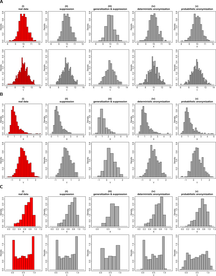
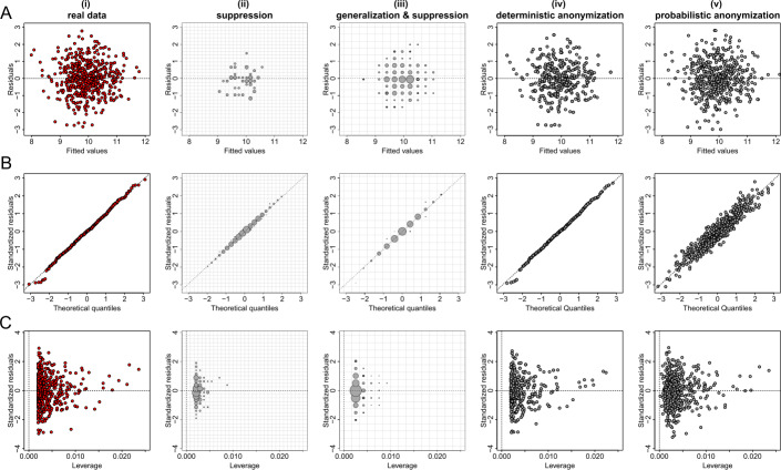
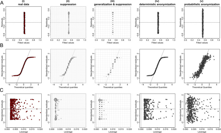
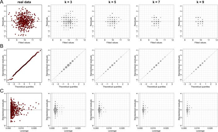
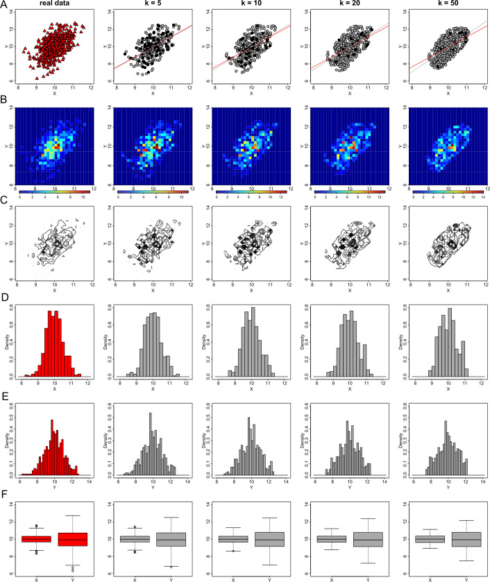
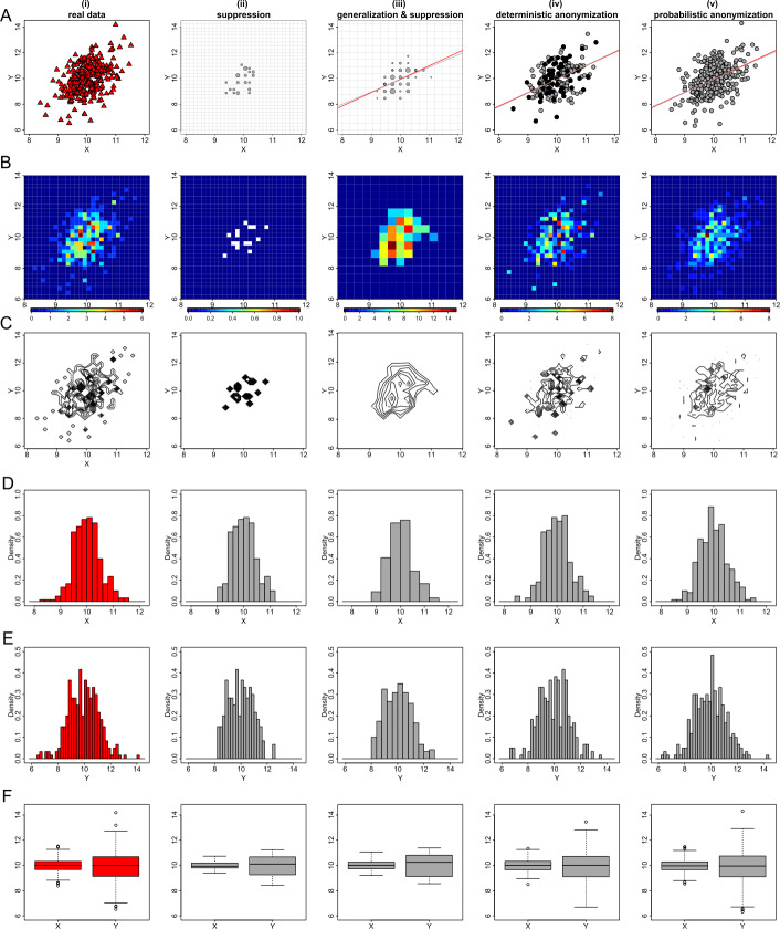
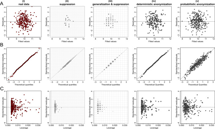
Data visualizations are a valuable tool used during both statistical analysis and the interpretation of results as they graphically reveal useful information about the structure, properties and relationships between variables, which may otherwise be concealed in tabulated data. In disciplines like medicine and the social sciences, where collected data include sensitive information about study participants, the sharing and publication of individual-level records is controlled by data protection laws and ethico-legal norms. Thus, as data visualizations - such as graphs and plots - may be linked to other released information and used to identify study participants and their personal attributes, their creation is often prohibited by the terms of data use. These restrictions are enforced to reduce the risk of breaching data subject confidentiality, however they limit analysts from displaying useful descriptive plots for their research features and findings. Here we propose the use of anonymization techniques to generate privacy-preserving visualizations that retain the statistical properties of the underlying data while still adhering to strict data disclosure rules. We demonstrate the use of (i) the well-known k-anonymization process which preserves privacy by reducing the granularity of the data using suppression and generalization, (ii) a novel deterministic approach that replaces individual-level observations with the centroids of each k nearest neighbours, and (iii) a probabilistic procedure that perturbs individual attributes with the addition of random stochastic noise. We apply the proposed methods to generate privacy-preserving data visualizations for exploratory data analysis and inferential regression plot diagnostics, and we discuss their strengths and limitations.

Keywords: Anonymization; Data visualizations; Disclosure control; Privacy protection; Sensitive data.

Figure 1

Privacy-preserving histograms. Figures (A), (B) and (C) show the histograms of X (top rows) and Y (bottom rows) from datasets D1, D2 and D3 respectively. From left to right we demonstrate (i) the histograms of the actual variables; (ii) the histograms of the variables after suppressing any bins with less than three counts; (iii) the histograms of the variables after generalizing the variables into bins based on wider intervals and suppressing any bins with less than three counts; (iv) the histograms of the scaled centroids of each 3-nearest neighbours; (v) the histograms of the variables with added noise of variance equal to 6.25% of the true variance. Note that the vertical axis represents the frequency density which is the frequency of each bin divided by its width

Figure 2

Privacy-preserving scatter plots. Figures (A), (B) and (C) show the scatter plots of X and Y from datasets D1, D2 and D3 respectively. From left to right we demonstrate: (i) the scatter plots of the actual variables; (ii) the scatter plots of the data aggregated in a 30 by 30 density grid matrix and suppressing any grids with density less than three counts; (iii) the scatter plots of the data aggregated in a 15 by 15 density grid matrix (i.e. additional generalization) and suppressing any grids with density less than three counts; (iv) the scatter plots of the scaled centroids of each 3-nearest neighbours obtained by deterministic anonymization; (v) the scatter plots of noisy X and Y obtained by addition of random stochastic noise in each variable, of variance equal to 6.25% of the true variability. Notes: Each data point in panels (ii)–(iii) is located at the center of the grid and its size corresponds to the number of observations in the grid. The grids are shown with transparent lines. Panels (ii)–(iii) in Figure (A) include the actual linear trend line of X and Y (red) and the weighted linear trend line of the k-anonymized data (grey). Panels (iv)–(v) in Figure (A) include the linear trend lines of actual (red) and anonymized (grey) X and Y variables. The black dots in panels (iv) indicate the positions where more than one centroids are identically placed

Figure 3

Privacy-preserving heat map and contour plots. Figures (A), (B) and (C) show the heat map (top rows) and contour (bottom rows) plots of X and Y from datasets D1, D2 and D3 respectively. From left to right we demonstrate the plots produced by: (i) the actual 30 by 30 density grid matrix; (ii) the actual 30 by 30 density grid matrix but suppressing any grids with density less than three counts; (iii) a generalized to 15 by 15 density grid matrix and suppressing any grids with density less than three counts; (iv) a 30 by 30 density grid matrix of deterministically anonymized variables using the value of $k=3$ when locating the k-nearest neighbours; (v) a 30 by 30 density grid matrix of probabilistically anonymized variables generated by adding random noise to the actual variables, of variance equal to 6.25% of their actual variance. Note that the colour scale differs between the different heat map plots

Figure 4

Privacy-preserving box plots. Figures (A), (B) and (C) show the box plots of X and Y from datasets D1, D2 and D3 respectively. From left to right we demonstrate: (i) the actual box plots of the variables; (ii) the data are aggregated in a 30 by 30 density grid matrix, any grids with density less than three counts are suppressed, and the box plots for the observations that are exist in the remaining grids are displayed; (iii) the data are aggregated in a 15 by 15 density grid matrix (i.e. further generalization), any grids with density less than three counts are suppressed, and the box plots for the observations that are exist in the remaining grids are displayed; (iv) the box plots of the scaled centroids of each 3-nearest neighbours obtained by deterministic anonymization; (v) the box plots of noisy variables obtained by addition of random stochastic noise in each variable, of variance equal to 6.25% of the true variability

Figure 5

Privacy-preserving regression diagnostic plots of data from dataset D1. (A) Residuals against fitted values; (B) Normal QQ plots; (C) Residuals against leverage. From left to right we demonstrate the plots: (i) for real regression outcomes; (ii) the regression outcomes aggregated in a 30 by 30 density grid matrix and suppressing any grids with density less than three counts; (iii) the regression outcomes aggregated in a 15 by 15 density grid matrix and suppressing any grids with density less than three counts; (iv) the scaled centroids of each 3-nearest neighbours of the regression outcomes obtained by deterministic anonymization; (v) the noisy regression outcomes obtained by probabilistic anonymization. Note that for plots B and C we use the standardized residuals that are the residuals divided by their standard deviation

Figure 6

Privacy-preserving regression diagnostic plots of data from dataset D2. (A) Residuals against fitted values; (B) Normal QQ plots; (C) Residuals against leverage. From left to right we demonstrate the plots: (i) for real regression outcomes; (ii) the regression outcomes aggregated in a 30 by 30 density grid matrix and suppressing any grids with density less than three counts; (iii) the regression outcomes aggregated in a 15 by 15 density grid matrix and suppressing any grids with density less than three counts; (iv) the scaled centroids of each 3-nearest neighbours of the regression outcomes obtained by deterministic anonymization; (v) the noisy regression outcomes obtained by probabilistic anonymization. Note that for plots B and C we use the standardized residuals that are the residuals divided by their standard deviation

Figure 7

Privacy-preserving regression diagnostic plots of data from dataset D3. (A) Residuals against fitted values; (B) Normal QQ plots; (C) Residuals against leverage. From left to right we demonstrate the plots: (i) for real regression outcomes; (ii) the regression outcomes aggregated in a 30 by 30 density grid matrix and suppressing any grids with density less than three counts; (iii) the regression outcomes aggregated in a 15 by 15 density grid matrix and suppressing any grids with density less than three counts; (iv) the scaled centroids of each 3-nearest neighbours of the regression outcomes obtained by deterministic anonymization; (v) the noisy regression outcomes obtained by probabilistic anonymization. Note that for plots B and C we use the standardized residuals that are the residuals divided by their standard deviation

Figure 8

The effect of parameter k of the k-anonymization method on exploratory data visualizations. From left to right we demonstrate the effect of k for the values of 1 (this is equivalent to the real data), 3, 5, 7 and 9 on generating privacy-preserving scatter plots (A), heat map plots (B), contour plots (C), histograms of X (D) and Y (E), and box plots (F)

Figure 9

The effect of parameter k of the k-anonymization method on exploratory data visualizations with additional generalization. From left to right we demonstrate the effect of k for the values of 1 (this is equivalent to the real data), 3, 5, 7 and 9 on generating privacy-preserving scatter plots (A), heat map plots (B), contour plots (C), histograms of X (D) and Y (E), and box plots (F)

Figure 10

The effect of parameter k of the k-anonymization method on regression plot diagnostics. From left to right we demonstrate the effect of k for the values of 1 (this is equivalent to the real data), 3, 5, 7 and 9 on generating privacy-preserving residuals vs fitted values plots (A), normal QQ plots (B), and standardized residuals vs leverage (C)

Figure 11

The effect of parameter k of the k-anonymization method on regression plot diagnostics with additional generalization. From left to right we demonstrate the effect of k for the values of 1 (this is equivalent to the real data), 3, 5, 7 and 9 on generating privacy-preserving residuals vs fitted values plots (A), normal QQ plots (B), and standardized residuals vs leverage (C)

Figure 12

The effect of parameter k of the deterministic anonymization method on exploratory data visualizations. From left to right we demonstrate the effect of k for the values of 1 (this is equivalent to the real data), 5, 10, 20 and 50 on generating privacy-preserving scatter plots (A), heat map plots (B), contour plots (C), histograms of X (D) and Y (E), and box plots (F)

Figure 13

The effect of parameter k of the deterministic anonymization method on regression plot diagnostics. From left to right we demonstrate the effect of k for the values of 1 (this is equivalent to the real data), 5, 10, 20 and 50 on generating privacy-preserving residuals vs fitted values plots (A), normal QQ plots (B), and standardized residuals vs leverage (C)

Figure 14

The effect of parameter q of the probabilistic anonymization method on exploratory data visualizations. From left to right we demonstrate the effect of q for the values of 0 (this is equivalent to the real data), 0.1, 0.5, 1 and $\sqrt{2}$ on generating privacy-preserving scatter plots (A), heat map plots (B), contour plots (C), histograms of X (D) and Y (E), and box plots (F)

Figure 15

The effect of parameter q of the probabilistic anonymization method on regression plot diagnostics. From left to right we demonstrate the effect of q for the values of 0 (this is equivalent to the real data), 0.1, 0.5, 1 and $\sqrt{2}$ on generating privacy-preserving residuals vs fitted values plots (A), normal QQ plots (B), and standardized residuals vs leverage (C)

Figure 16

The performance of the techniques applied in a sample of 50 observations. From top to bottom we demonstrate the scatter plots (A), heat map plots (B), contour plots (C), histograms of X (D) and Y (E), and box plots (F) for real data (i), suppressed data (ii), generalized and suppressed data (iii), deterministically anonymized data (iv) and probabilistic anonymized data (v)

Figure 17

The performance of the techniques applied in a sample of 50 observations. From top to bottom we demonstrate the residuals vs fitted values plots (A), normal QQ plots (B), and standardized residuals vs leverage plots (C) for real regression outcomes (i), suppressed regression outcomes (ii), generalized and suppressed regression outcomes (iii), deterministically anonymized regression outcomes (iv) and probabilistic anonymized regression outcomes (v)

Figure 18

The performance of the techniques applied in a sample of 100 observations. From top to bottom we demonstrate the scatter plots (A), heat map plots (B), contour plots (C), histograms of X (D) and Y (E), and box plots (F) for real data (i), suppressed data (ii), generalized and suppressed data (iii), deterministically anonymized data (iv) and probabilistic anonymized data (v)

Figure 19

The performance of the techniques applied in a sample of 100 observations. From top to bottom we demonstrate the residuals vs fitted values plots (A), normal QQ plots (B), and standardized residuals vs leverage plots (C) for real regression outcomes (i), suppressed regression outcomes (ii), generalized and suppressed regression outcomes (iii), deterministically anonymized regression outcomes (iv) and probabilistic anonymized regression outcomes (v)

Figure 20

The performance of the techniques applied in a sample of 300 observations. From top to bottom we demonstrate the scatter plots (A), heat map plots (B), contour plots (C), histograms of X (D) and Y (E), and box plots (F) for real data (i), suppressed data (ii), generalized and suppressed data (iii), deterministically anonymized data (iv) and probabilistic anonymized data (v)

Figure 21

The performance of the techniques applied in a sample of 300 observations. From top to bottom we demonstrate the residuals vs fitted values plots (A), normal QQ plots (B), and standardized residuals vs leverage plots (C) for real regression outcomes (i), suppressed regression outcomes (ii), generalized and suppressed regression outcomes (iii), deterministically anonymized regression outcomes (iv) and probabilistic anonymized regression outcomes (v)

References

1. Healy K, Moody J. Data visualization in sociology. Annu Rev Sociol. 2014;40:105–128. doi: 10.1146/annurev-soc-071312-145551. - DOI - PMC - PubMed
1. O’Donoghue SI, Gavin A-C, Gehlenborg N, Goodsell DS, Hériché J-K, Nielsen CB, North C, Olson AJ, Procter JB, Shattuck DW, Walter T, Wong B. Visualizing biological data–now and in the future. Nat Methods. 2010;7:2–4. doi: 10.1038/nmeth.f.301. - DOI - PubMed
1. O’Donoghue SI, Baldi BF, Clark SJ, Darling AE, Hogan JM, Kaur S, Maier-Hein L, McCarthy DJ, Moore WJ, Stenau E, Swedlow JR, Vuong J, Procter JB. Visualization of biomedical data. Annu Rev Biomed Data Sci. 2018;1(1):275–304. doi: 10.1146/annurev-biodatasci-080917-013424. - DOI
1. Matejka J, Fitzmaurice G. Proceedings of the 2017 CHI conference on human factors in computing systems. New York: ACM; 2017. Same stats, different graphs: generating datasets with varied appearance and identical statistics through simulated annealing; pp. 1290–1294.
1. Morrison J, Vogel D. The impacts of presentation visuals on persuasion. Inf Manag. 1998;33(3):125–135. doi: 10.1016/S0378-7206(97)00041-4. - DOI