Estimating density limits for walking pedestrians keeping a safe interpersonal distancing

Abstract

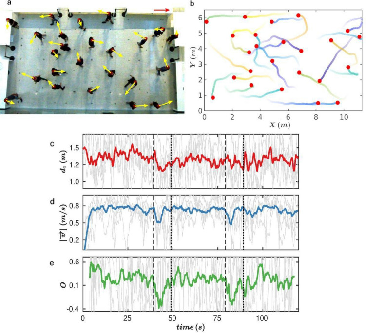
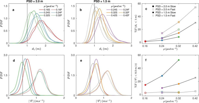
With people trying to keep a safe distance from others due to the COVID-19 outbreak, the way in which pedestrians walk has completely changed since the pandemic broke out^1,2. In this work, laboratory experiments demonstrate the effect of several variables-such as the pedestrian density, the walking speed and the prescribed safety distance-on the interpersonal distance established when people move within relatively dense crowds. Notably, we observe that the density should not be higher than 0.16 pedestrians per square meter (around 6 m² per pedestrian) in order to guarantee an interpersonal distance of 1 m. Although the extrapolation of our findings to other more realistic scenarios is not straightforward, they can be used as a first approach to establish density restrictions in urban and architectonic spaces based on scientific evidence.

Figure 1

Experimental setup, pedestrian trajectories and time series. (a) Snapshot of an experiment with 24 people walking at a slow pace for a Prescribed Safety Distance (PSD) of 1.5 m. Yellow arrows correspond to the instantaneous velocities based on the scale indicated by the red vector (1 ms⁻¹) at the right top of the panel. (b) Example of the trajectories followed by pedestrians during the 5 s previous to the snapshot shown in a. The colour of paths fades out with elapsed time (representation of the entire trajectories is given Fig. 5d, “Methods” section). (c–e) Temporal evolution of (c) the distances to the nearest pedestrian d1, (d) velocity modulus and (e) persistence in movement direction O for the same experiment shown in a, b. For each pedestrian, we calculated O as cos[θi(t + τ) − θi(t)] for a time delay of τ = 2 s, where θ(t) represents the direction of pedestrian velocity at time t, calculated as atan(Vy/Vx). Light grey lines represent the value of each magnitude for 5 chosen pedestrians, whereas solid coloured lines represent the value of the variable averaged over the total number of pedestrians in the experiment (24 in this case). Vertical dashed and dotted lines indicate the times at which the change in the movement direction start and finish, respectively.

Figure 2

Minimum distances to the nearest neighbour and pedestrian velocities. (a, b) Probability density functions (PDFs) of the distances to the nearest pedestrian (d₁) for a Prescribed Safety Distance (PSD) of (a) 2 m and (b) 1.5 m for different crowd densities, as indicated in the legend. Solid lines correspond to slow walking speed (S in the legend) and dotted lines to fast walking speed (F in the legend). (c) percentage of time that, on average, a pedestrian has a neighbour closer than 1 m, as a function of the crowd density for the different experimental conditions explored (see legend). (d, e) PDFs of velocity modules for different densities for (d) PSD = 2 m and (e) PSD = 1.5 m. Same legend as in (a, b). (f) Percentage of time that the velocity of a pedestrian is below 0.5 m/s for different PSD and walking speed values. Same legend as (c). Vertical dashed line in (a, b, d, e) provide a reference to help in the interpretation of figures (c, f).

Figure 3

Exposure times and persistence of movement direction. (a, b) Distributions of exposure time periods (t_exp) during which two pedestrians are uninterruptedly closer than 1.5 m. Probability density functions (PDFs) of t_exp when the prescribed safety distance is (a) 2 m and (b) 1.5 m for different densities, as indicated in the legend. Solid lines correspond to slow walking speed (S in the legend) and dotted lines to fast walking speed (F in the legend). (c) Number of times that a pedestrian is uninterruptedly closer than 1.5 m to another during a t_exp greater or equal to 2 s, as a function of density, for the experimental conditions indicated in the legend. The number of events recorded in each condition is normalized by the number of pedestrians within the room and the total duration (in minutes) of the test. (d) PDFs of t_exp re-scaled by the pedestrian average speed modulus measured at each experiment. Colours are the same for experiments with the same density; solid lines correspond to slow walking speed and dotted lines to fast walking speed.

Figure 4

Persistence of movement direction. (a–c) Probability density functions (PDFs) of the persistence of movement direction O for an experiment in which ρ = 0.24 ped m⁻², the prescribed safety distance (PSD) was 2 m, and the walking speed was fast (see Number 4 in Table 1). Different colours are used to represent distributions with different values of τ as indicated in the legend. (b, c) ‹O› as a function of τ for (b) PSD = 2 m and (c) PSD = 1.5 m for different densities values as indicated in the legend. (d) ‹O› as a function of the selected τ value re-scaled by the average speed modulus measured for each experimental condition. Solid lines correspond to slow walking speed (WS) and dotted lines to fast walking speed.

Figure 5

(Methods) | Experimental scenario. (a) Side view of the arena delimited by several tables. In the far right corner of the arena the reference checkboard (1.8 m height) can be seen. At the top of the picture, the camera is hanging at around 12 m. (b) Top view of the experimental scenario delimited by tables. On the floor, the different crosses marking the initial positions for the experiments with a prescribed distance of 2 m (black spots) and 1.5 m (green spots) can be observed. (c) Picture in which pedestrians wearing dark clothes, masks, and a red hat, are participating in one of the drills. (d) Set of pedestrians’ trajectories for the same experiment as in Fig. 1 (24 people walking at a slow pace for a prescribed safety distance of 1.5 m). Horizontal and vertical axes label the distance from the bottom-left corner of the scene, in meters.

References

1. Pouw CA, Toschi F, van Schadewijk F, Corbetta A. Monitoring physical distancing for crowd management: real-time trajectory and group analysis. PLoS One. 2020;15(10):e0240963. doi: 10.1371/journal.pone.0240963. - DOI - PMC - PubMed
1. Seres, G., Balleyer, A. H., Cerutti, N., & Friedrichsen, J. Face mask use and physical distancing before and after mandatory masking: evidence from public waiting lines. Available at SSRN 3641367 (2020). - PMC - PubMed
1. https://www.who.int/emergencies/diseases/novel-coronavirus-2019/advice-f....
1. Helbing D, Molnar P. Social force model for pedestrian dynamics. Phys. Rev. E. 1995;51:4282. doi: 10.1103/PhysRevE.51.4282. - DOI - PubMed
1. Helbing D, Farkas I, Vicsek T. Simulating dynamic features of escape panic. Nature. 2000;407:487–490. doi: 10.1038/35035023. - DOI - PubMed
Publication types
LinkOut - more resources