Metropolitan age-specific mortality trends at borough and neighborhood level: The case of Mexico City

Abstract

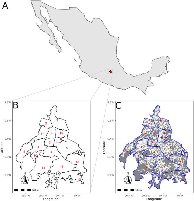
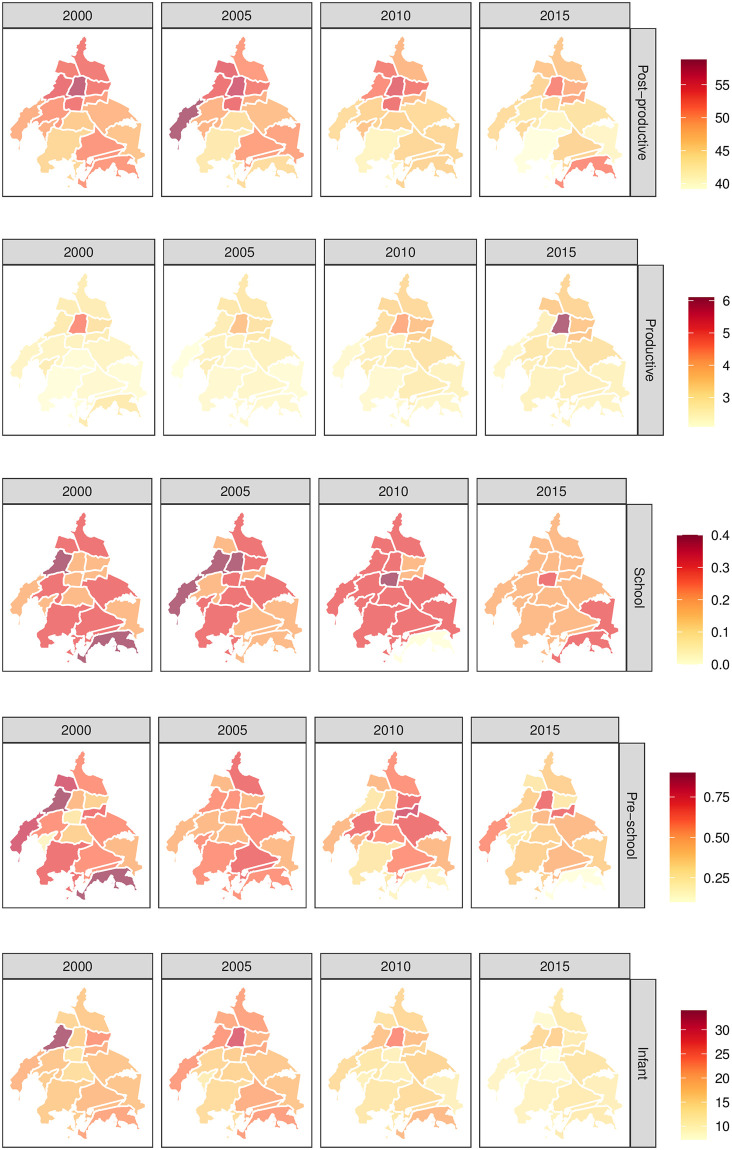
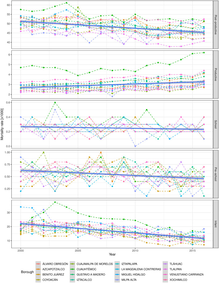
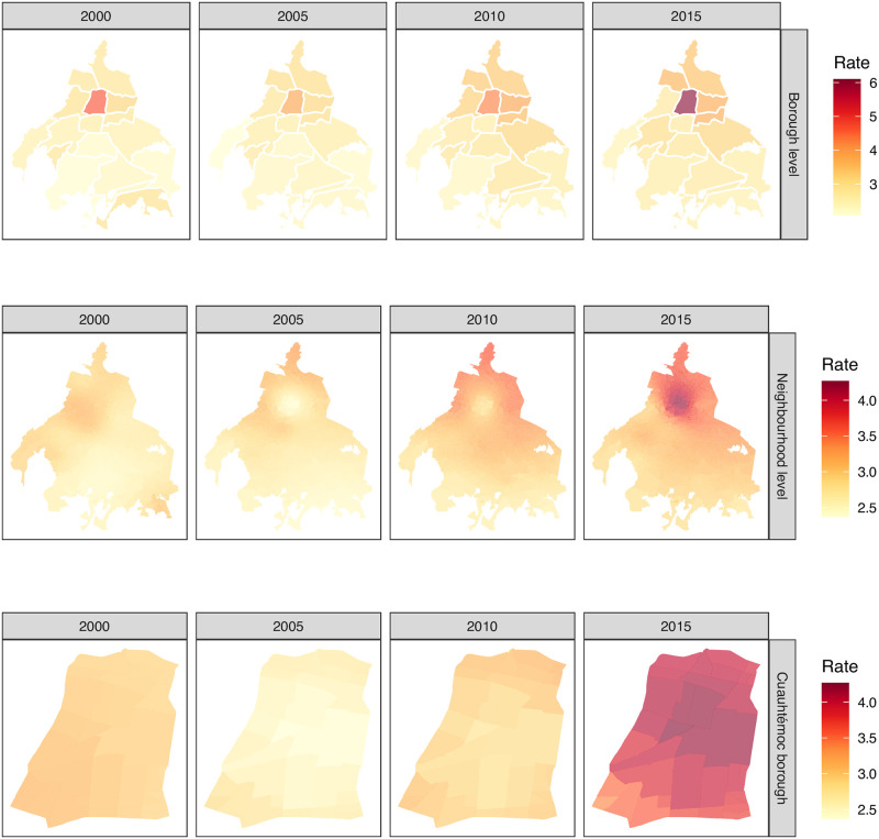
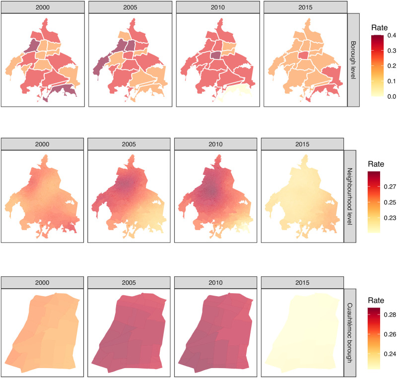
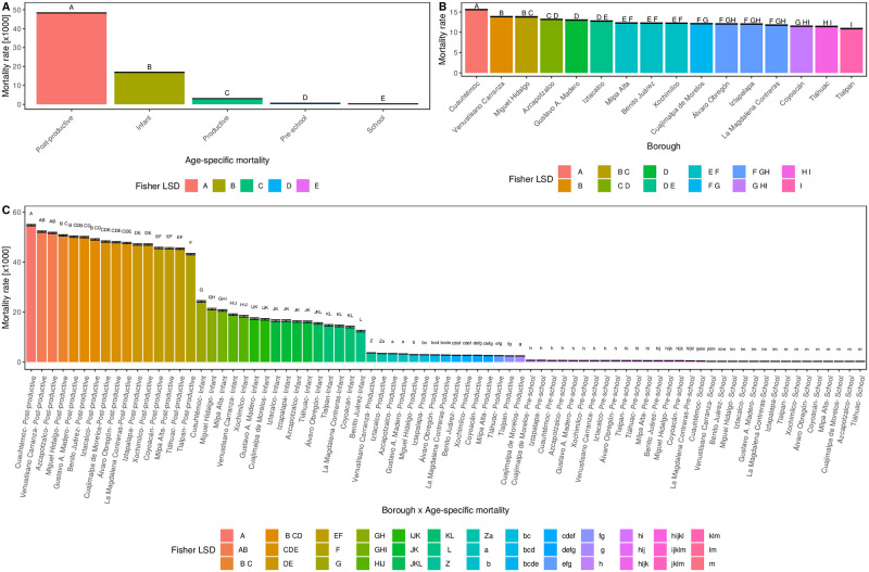
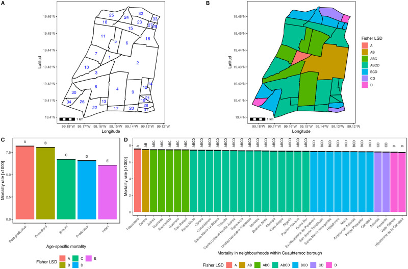
Understanding the spatial and temporal patterns of mortality rates in a highly heterogeneous metropolis, is a matter of public policy interest. In this context, there is no, to the best of our knowledge, previous studies that correlate both spatio-temporal and age-specific mortality rates in Mexico City. Spatio-temporal Kriging modeling was used over five age-specific mortality rates (from the years 2000 to 2016 in Mexico City), to gain both spatial (borough and neighborhood) and temporal (year and trimester) data level description. Mortality age-specific patterns have been modeled using multilevel modeling for longitudinal data. Posterior tests were carried out to compare mortality averages between geo-spatial locations. Mortality correlation extends in all study groups for as long as 12 years and as far as 13.27 km. The highest mortality rate takes place in the Cuauhtémoc borough, the commercial, touristic and cultural core downtown of Mexico City. On the contrary, Tlalpan borough is the one with the lowest mortality rates in all the study groups. Post-productive mortality is the first age-specific cause of death, followed by infant, productive, pre-school and scholar groups. The combinations of spatio-temporal Kriging estimation and time-evolution linear mixed-effect models, allowed us to unveil relevant time and location trends that may be useful for public policy planning in Mexico City.

Fig 1. Mexico City study area.

A) The map of Mexico shows the location of Mexico City (in red), formerly known as Distrito Federal, one of the 32 states of Mexico which is located in the central area. B) Borough level description of the 16 cases (in numbers) corresponding to: 1. Álvaro Obregón, 2. Azcapotzalco, 3. Benito Juárez, 4. Coyoacán, 5. Cuajimalpa de Morelos, 6. Cuauhtémoc, 7. Gustavo A. Madero, 8. Iztacalco, 9. Iztapalapa, 10. La Magdalena Contreras, 11. Miguel Hidalgo, 12. Milpa Alta, 13. Tláhuac, 14. Tlalpan, 15. Venustiano Carranza and 16. Xochimilco. C) Neighborhood level description. Blue lines describe borough limits, whereas white lines at neighborhood areas (in gray). Red dots depict borough calculated centroids. In panels A and B, the scale bar and north arrow are also included. Notice that some boroughs have a dense neighborhood description in comparison.

Fig 2. Spatial age-specific mortality rates in Mexico City’s boroughs.

Each row corresponds to a particular age-specific mortality rate, i.e., Post-productive (x ≥ 64 years old), Productive (14 ≤ x < 64 years old), School (4 ≤ x < 14 years old), Pre-school (1 ≤ x < 4 years old) and Infant (x < 1 years old). Each column stands for the selected years 2000, 2005, 2010 and 2015 from the total yearly available period 2000 to 2016. Mexico City boroughs are treated as a the unit area and color coded according to the corresponding mortality rate, which make them comparable by row. Interestingly, notice the different mortality rate ranges (color bars) depending on the age-specific group of analysis. Polygon shapefiles files can be freely downloaded at INEGI’s website [40], whereas mortality data from SEDESA [52].

Fig 3. Temporal age-specific mortality rates in Mexico City’s boroughs.

Each panel corresponds to an age-specific mortality rate, i.e., Post-productive (x ≥ 64 years old), Productive (14 ≤ x < 64 years old), School (4 ≤ x < 14 years old), Pre-school (1 ≤ x < 4 years old) and Infant (x < 1 years old). All panels include complete age-specific mortality rates records by year from 2000 up to 2016 (in colour points) from SEDESA [52]. Color points stand for one of the 16 boroughs in Mexico City longitudinal mortality rate data. Borough data have been joined by their corresponding color dashed lines, whereas complete age-specific panel has been modeled by a linear regression (intercept and slope, blue line) with its respective standard deviation (grey area), to get a clear picture of the time evolution pattern. Interestingly, as the years pass, the mortality rate time evolution seems to diminish for Infant and Post-productive groups, whereas the Productive age-specific counterpart tends to increase.

Fig 4. Three levels of granularity for productive mortality rate in Mexico City.

First one, productive mortality rate original data description at borough level (panel A). Second one, productive mortality rate kriged data description at the neighborhood level is presented in panel B. In panel C, it is presented a zoom-in at a second description level for Cuauhtémoc borough. Interestingly, this is the borough with the highest productive mortality rate no matter the selected year (2000, 2005, 2010 or 2015), according to panel A and B (central borough in red). However, the mortality rate is not homogeneous at the neighborhood level, as depicted by the kriged values presented in panel C for the different years. Polygon shapefiles files can be freely downloaded at INEGI’s website [40].

Fig 5. Three levels of granularity for school mortality rate in Mexico City.

First, school mortality rate original data description is presented at borough level (panel A). Second, school mortality rate kriged data description at the neighborhood level is presented at panel B. In panel C, it is presented a zoom-in at the neighborhood level for the Cuauhtémoc borough. Interestingly, the school mortality rate for this borough increments from the year 2000 to 2005, while it reduces from 2005 to 2015 according to panels A and B, whereas the city’s southeast area shows an increment from 2005 to 2015. However, the mortality rate is neither homogeneous nor constant at the neighborhood level, as depicted by the kriged values presented in panel C. Polygon shapefiles files can be freely downloaded at INEGI’s website [40].

Fig 6. Posterior mortality rate test results at borough level for Mexico City.

Fisher’s Least Significant Difference (LSD) tests were performed over the estimated age-specific mean mortality rate, according to model description in Eqs ((1)–(4)). In panels, Mexico City Fisher’s LSD test results for: A) Age-specific mortality, B) Borough level, and, C) Borough × Age-specific interaction. The LSD group mean test results are presented as bar-plots with their corresponding standard deviation bar and mean group letters (A, B, C …), where bars that share at least a single letter, are not statistically different after Bonferroni multiple test correction (p > 0.05). Interestingly, mortality rates is mainly composed by age-specific contribution when compared to Borough impact. In addition, Borough × Age-specific interaction retains the mortality age-specific rate pattern, but, it is modulated by the borough contribution.

Fig 7. Posterior neighborhood mortality test results zoom-in at Cuauhtémoc borough in Mexico City.

A) Cuauhtémoc borough is divided into its 34 neighborhoods. Numbers are ordered from the highest (1) to the lowest (34) model estimated neighborhood fixed effect mortality mean according to Eqs (1)–(4) description: 1. Tabacalera, 2. Centro, 3. Juárez, 4. Doctores, 5. Buenavista, 6. Guerrero, 7. San Rafael, 8. Roma Norte, 9. Obrera, 10. Cuauhtémoc, 11. Santa María la Ribera, 12. Tránsito, 13. Centro Urbano Benito Juárez, 14. Esperanza, 15. Unidad Hab. Nonoalco Tlatelolco, 16. Morelos, 17. Buenos Aires, 18. Atlampa, 19. Vista Alegre, 20. Algarín, 21. Paulino Navarro, 22. Roma Sur, 23. Ex-hipódromo de Peralvillo, 24. San Simón Tolnáhuac, 25. Santa María Insurgentes, 26. Hipódromo, 27. Maza, 28. Ampl. Asturias, 29. Felipe Pescador, 30. Condesa, 31. Asturias, 32. Peralvillo, 33. Valle Gómez and 34. Hipódromo de la Condesa. B) Neighborhoods are filled according to the Fisher’s Least Significant Difference (LSD) group mean obtained at this level of representation. C) Age-specific Fisher’s LSD results within Cuauhtémoc borough. D) Fisher’s LSD neighborhood contribution. In all cases, capital letters stand for Fisher’s LSD groups, where bars that share at least a single letter, are not statistically different after Bonferroni multiple test correction (p > 0.05). Results are presented as ordered mean ± standard error estimation according to model description of Eqs (1)–(4). Notice that at this data level decomposition, the LSD group means are at the same mortality rate order, i.e., the age-specific group mean values are comparable to the different neighborhood contribution. In addition, age-specific mortality values do not overlap whereas, most of the neighborhoods within this specific borough, share a common LSD group.

References

1. Gaskin DJ, Roberts ET, Chan KS, McCleary R, Buttorff C, Delarmente BA. No man is an island: the impact of neighborhood disadvantage on mortality. Int J Environ Res Public Health. 2019;16(7):1265 10.3390/ijerph16071265 - DOI - PMC - PubMed
1. Gavurova B, Toth P. Preventable Mortality in Regions of Slovakia—Quantification of Regional Disparities and Investigation of the Impact of Environmental Factors. Int J Environ Res Public Health. 2019;16(8). 10.3390/ijerph16081382 - DOI - PMC - PubMed
1. Rodríguez-Sanz M, Gotsens M, dell?Olmo MM, Borrell C. Trends in mortality inequalities in an urban area: the influence of immigration. Int J Equity Health. 2019;18(1):37 10.1186/s12939-019-0939-9 - DOI - PMC - PubMed
1. Ayele DG, Zewotir TT. Childhood mortality spatial distribution in Ethiopia. J Appl Stat. 2016;43(15):2813–2828. 10.1080/02664763.2016.1144727 - DOI
1. Burke M, Heft-Neal S, Bendavid E. Sources of variation in under-5 mortality across sub-Saharan Africa: a spatial analysis. Lancet Public Health. 2016;4(12):e936–e945. - PubMed
LinkOut - more resources