The Divider Assay is a high-throughput pipeline for aggression analysis in Drosophila

Abstract

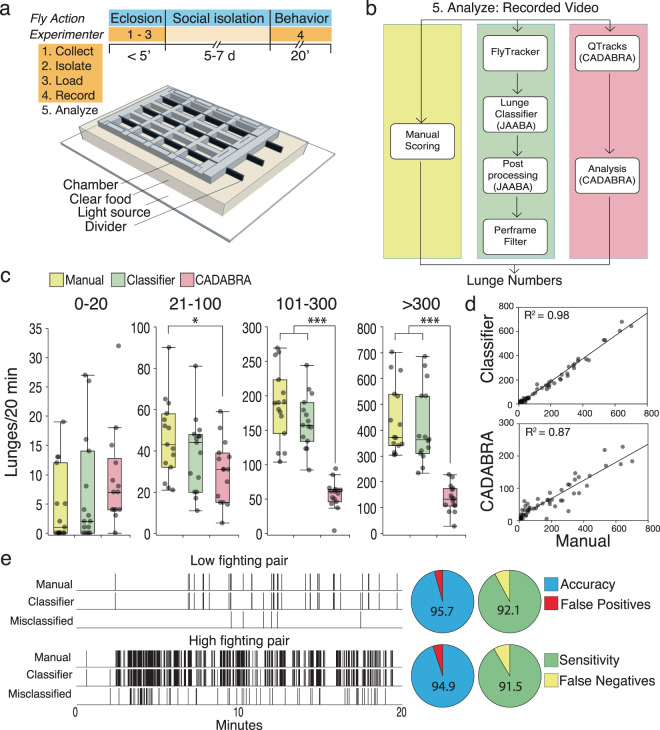
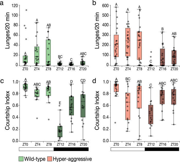
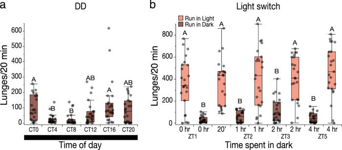
Aggression is a complex social behavior that remains poorly understood. Drosophila has become a powerful model system to study the underlying biology of aggression but lack of high throughput screening and analysis continues to be a barrier for comprehensive mutant and circuit discovery. Here we developed the Divider Assay, a simplified experimental procedure to make aggression analysis in Drosophila fast and accurate. In contrast to existing methods, we can analyze aggression over long time intervals and in complete darkness. While aggression is reduced in the dark, flies are capable of intense fighting without seeing their opponent. Twenty-four-hour behavioral analysis showed a peak in fighting during the middle of the day, a drastic drop at night, followed by re-engagement with a further increase in aggression in anticipation of the next day. Our pipeline is easy to implement and will facilitate high throughput screening for mechanistic dissection of aggression.

Fig. 1. Divider Assay for precise quantification of aggression over a broad range of fighting intensities.

a Schematic of the Divider Assay setup and experimental time line. Collecting, isolating, and loading flies are done in one step under 5 min. Flies are then isolated on clear food until they are videotaped. b Recorded video analysis can be done manually (yellow), with a newly developed JAABA-based classifier to precisely score lunges (green), or with existing CADABRA software (red). c Sixty pairs of flies with lunges ranging from 0 to 700 were analyzed manually, with a new JAABA-based classifier, and CADABRA. For this analysis, four groups of fighting intensities were chosen: 0–20, 21–100, 101–300, and >300 lunges. The JAABA-based classifier performed close to the gold standard with no significant differences in any group (Kruskal–Wallis ANOVA with Dunn’s test and Bonferroni correction 0–20, p = 1.0; 21–100, p = 0.55; 101–300, p = 0.75; >300, p = 1.0, n = 15 per group). CADABRA tended to overscore low fighting flies, but significantly underscored high fighting pairs (Kruskal–Wallis ANOVA with Dunn’s test and Bonferroni correction, 0–20: p = 0.08, n = 14; 21–100: p = 0.03; 101–300: p < 0.0001; >300: p < 0.0001, n = 15 per group) (see also Supplementary Fig. 1, for Gardner–Altman estimation plots). d Regression analysis between manual scoring and classifier (R² = 0.98, p < 0.0001, n = 60) or CADABRA (R² = 0.87, p < 0.0001, n = 59) are both highly significant. e Misclassified lunges with the JAABA-based classifier occur at low frequency in both low and high fighting pairs (false positives ~5% and false negatives ~8%). Boxplots show the median, first and third quartiles as boxes, with whiskers representing the 5 and 95% intervals.

Fig. 2. Increased space decreases aggression.

a Lunge numbers decrease with increasing height of the square arenas for low fighting control strain. There is no difference between 4.5 and 3.5 mm, which is approximately the height of a fly raised on its hindlegs (nonparametric Steel method with 4.5 mm as control height, p = 0.34). As the height of the arena increases to 7.5 and 11 mm lunge numbers statistically significantly decrease (nonparametric Steel method compared to 4.5 mm as a control, 7.5^CS, p = 0.001; 11^CS, p < 0.001). b For hyper-aggressive flies, the decrease only became statistically significant at 11 mm (nonparametric Steel method compared to 4.5 mm height as control, 3.5^Aggr, p = 1; 7.5^Aggr, p = 0.11; 11^Aggr, p = 0.005, n = 22–24 per group). c, d Increasing the surface area of the arenas ~5 to 13-fold by doubling or tripling the width of the arena also decreased aggression. In both low and high aggression strains, the difference becomes statistically significant when the arena width is tripled (nonparametric Steel method with 1× surface area as the control, 1×^CS vs. 5×^CS, p = 0.07; vs. 13×^CS p = 0.002; 1×^Aggr vs. 5×^Aggr, p = 0.07; vs. 13×^Aggr p = 0.001, n = 17–24 per group). Boxplots show the median, first and third quartiles as boxes, with whiskers representing the 5 and 95% intervals.

Fig. 3. Old flies remain aggressive.

a Control flies peak by 5 days and decline after but some flies still fight by 30 days of age. There is no significant difference in fighting between 5- or 10-day-old flies, but all other ages are significantly lower than 5-day-old flies (nonparametric Steel method with the 5-day-old as a control, 5d^CS vs. 1d^CS, p = 0.0002; 5d^CS vs. 2d^CS, p = 0.0011; 5d^CS vs. 3d^CS, p = 0.57; 5d^CS vs. 10d^CS, p = 0.50; 5d^CS vs. 30d^CS, p = 0.0017, n = 19-24 per group). b Compared to control flies hyper-aggressive flies already fight a lot by 2 days of age, but further significantly increase in aggression by 5 days. Even at 30 days, these flies still lunge more than 150 times in 20 min (nonparametric Steel method with the 5-day-old as a control, 5d^Aggr vs. 1d^Aggr, p < 0.0001; 5d^Aggr vs. 2d^Aggr, p = 0.23; 5d^Aggr vs. 3d^Aggr, p = 0.92; 5d^Aggr vs. 10d^Aggr, p = 0.19; 5d^Aggr vs. 30d^Aggr, p = 0.06, n = 21–24 per group). Boxplots show the median, first and third quartiles as boxes, with whiskers representing the 5 and 95% intervals.

Fig. 4. Comparison of the Divider Assay with other aggression assays.

a Lunge numbers (left plot) and latencies to lunge (right plot) in two established assays, the Colosseum assay and the Arena Assay, show similar differences between control and hyper-aggressive strains as in the Divider Assay. In all assays the differences are statistically significant (Wilcoxon rank-sum test, n = 22–24 per group). b Overview of the parameter differences in the three assay systems: age, fly handling, presence or absence of food, method of analysis, and duration of the experiment are different in the three assays. The Divider Assay is easiest to run because flies are collected, isolated, and loaded in a single step and lunges are analyzed in an automated manner. c Analysis of lunges in 2 min time bins shows significant differences in lunge numbers between the low and high aggression strains (Wilcoxon rank-sum test, 1–2 min, p = 0.001; 5–6 min, p = 0.0009; 10–11 min, p < 0.0001; 19–20 min, p < 0.0001, n = 24). d Plot of the median differences between the low (green squares) and high (red squares) aggression strains The largest difference between the two strains occurs at the 2 min bin at 10 min of videotaping. Median lunge numbers decrease significantly by 20 min in the hyper-aggressive strain (Wilcoxon rank-sum test, Aggr^10′ vs. Aggr^20′, p = 0.03, n = 24). In the low aggression strain median lunge number keep increasing over time and reach the highest levels in the last 2 min time bin (Wilcoxon rank-sum test, CS^2′ vs. CS^20′, p = 0.0^2′, Wilcoxon rank-sum test, n = 24). e Fighting frequencies, the percentage of pairs that show clear dominance between both flies, correlates very significantly with lunge numbers as previously shown (R² = 0.84, p < 0.0001, 10–12 fighting pairs per data point, n = 213). Boxplots show the median, first and third quartiles as boxes, with whiskers representing the 5 and 95% intervals.

Fig. 5. Mean Aggression Score (MAS) does not measure aggression.

a Median (line in the box) and average lunge (green square) numbers of 47 DGRP strains that were previously analyzed for MAS (blue circles). None of the strains have lunge numbers above 15 in 20 min interval (very low or no aggression in the range of CS). MAS varies 20-fold from ~4 in the lowest strain to ~80 in the highest strain. b Regression analysis shows that both parameters—lunge number and MAS—are not correlated (R² = 0.0002, n = 12–24). c Average locomotion data over 20 min of the five DGRP strains with lowest MAS and five DGRP strains with the highest MAS compared to the low (green horizontal bar) aggression and hyper-aggressive (red horizontal bar) strains. Most of the DGRP strains have significantly lower locomotor activity than CS (nonparametric Steel method with CS as the control, 352, p = 0.35; 228, p = 0.33; 235, p = 0.0007; 356, p = 0.0054; 379, p = 0.30; 350, p = 0.0077; 358, p = 0.027; 321, p = 0.42; 306, p = 0.018; 324, p = 0.044; Aggr, p = 0.02). Boxplots show the median, first and third quartiles as boxes, with whiskers representing the 5 and 95% intervals.

Fig. 6. Aggression shows 24 h variation.

a Lunge number variation over the different times of the day. In the low aggression strain, lunge numbers are highest during the day with a trend to peak at ZT4. At night lunges decrease significantly and increase again in anticipation of the next day (Kruskal–Wallis ANOVA with Dunn’s test and Bonferroni correction, significant differences are denoted with letters, ZT16 vs. ZT8, p = 0.026; ZT12 vs. ZT0, p = 0.0018; ZT12 vs. ZT4, p = 0.0015; ZT16 vs. ZT0, p = 0.0002; ZT16 vs. ZT4, p = 0.0002, n = 20–24 pairs per time point). b The lunge number variation follows a similar pattern but is more pronounced in the hyper-aggressive strain (Kruskal–Wallis ANOVA with Dunn’s test and Bonferroni correction, ZT20 vs. ZT12, p = 0.018; ZT20 vs. ZT0, p = 0.017; ZT16 vs. ZT4, p = 0.015; ZT16 vs. ZT8, p = 0.017; ZT12 vs. ZT0, p < 0.0001; ZT12 vs. ZT4, p < 0.0001; ZT12 vs. ZT8, p < 0.0001, n = 24 pairs per time point). c The pattern of daily lunge number variation is similar to the variation in courtship index. In the low aggression strain, courtship is highest early in the day with a statistically significant decrease around noon, a steep drop at the beginning of the night, courtship then increases again in the middle of the night with a further although not significant increase in anticipation of the day (Kruskal–Wallis ANOVA with Dunn’s test and Bonferroni correction, ZT16 vs. ZT8, p = 0.026; ZT20 vs. ZT0, p = 0.0003; ZT16 vs. ZT0, p < 0.0001; ZT12 vs. ZT4, p = 0.0003; ZT12 vs. ZT8, p < 0.0001; ZT12 vs. ZT0, p < 0.0001, n = 15–22 pairs per time point). d The same pattern can be observed in the hyper-aggressive strain with peak courtship in the early morning, a statistically significant decrease at noon, a steep decrease in the beginning of the night with recovery later in the night (Kruskal–Wallis ANOVA with Dunn’s test and Bonferroni correction, ZT12 vs. ZT8, p = 0.019; ZT4 vs. ZT0, p = 0.0047; ZT12 vs. ZT0, p < 0.0001, n = 15–22 pairs per time point). Boxplots show the median, first and third quartiles as boxes, with whiskers representing the 5 and 95% intervals.

Fig. 7. Aggression under free-running conditions compared to the effect lights “ON” and “OFF”.

a Lunge number variations of the hyper-aggressive strain at different times of the day under free-running DD conditions (Kruskal–Wallis ANOVA with Dunn’s test and Bonferroni correction, CT0 vs. CT8, p = 0.0024; CT0 vs. CT4, p = 0.033; CT16 vs. CT8, p = 0.0009; CT16 vs. CT4, p = 0.0154; CT20 vs. CT4, p = 0.0983; CT12 vs. CT4, p = 0.5288; CT20 vs. CT4, p = 0.7187, n = 20–24 pairs per time point). b Lunge numbers in flies that are run in light vs. dark at the beginning of the day significantly decrease strongly compared to flies run in light and flies kept in dark for 20 min and are then run in light (Kruskal–Wallis ANOVA with Dunn’s test and Bonferroni correction, ZT1^0L vs. ZT1^0D, p < 0.0001; ZT1^0L vs. ZT1^20′L, p = 1.000; ZT1^0D vs. ZT1^20′L, p < 0.0001, n = 24 pairs per time point). Increasing the dark treatment duration does not significantly increase lunge numbers of dark tested (Kruskal–Wallis ANOVA with Dunn’s test and Bonferroni correction, all dark comparisons, p = 1.000, n = 24 pairs per time point). Dark treatment followed by testing the flies in light leads to fully recovered lunge numbers (Kruskal–Wallis ANOVA with Dunn’s test and Bonferroni correction, all light comparisons, p = 1.000, n = 23–24 pairs per time point). Boxplots show the median, first and third quartiles as boxes, with whiskers representing the 5 and 95% intervals.

References

1. Vosshall LB. Into the mind of a fly. Nature. 2007;450:193–197. doi: 10.1038/nature06335. - DOI - PubMed
1. del Valle Rodriguez A, Didiano D, Desplan C. Power tools for gene expression and clonal analysis in Drosophila. Nat. Methods. 2011;9:47–55. doi: 10.1038/nmeth.1800. - DOI - PMC - PubMed
1. Venken KJ, Bellen HJ. Chemical mutagens, transposons, and transgenes to interrogate gene function in Drosophila melanogaster. Methods. 2014;68:15–28. doi: 10.1016/j.ymeth.2014.02.025. - DOI - PMC - PubMed
1. Gratz SJ, Rubinstein CD, Harrison MM, Wildonger J, O’Connor-Giles KM. CRISPR-Cas9 genome editing in Drosophila. Curr. Protoc. Mol. Biol. 2015;111:31.2.1–31.2.20. doi: 10.1002/0471142727.mb3102s111. - DOI - PMC - PubMed
1. Venken KJ, Simpson JH, Bellen HJ. Genetic manipulation of genes and cells in the nervous system of the fruit fly. Neuron. 2011;72:202–230. doi: 10.1016/j.neuron.2011.09.021. - DOI - PMC - PubMed
Publication types
LinkOut - more resources