Survey of spiking in the mouse visual system reveals functional hierarchy

Abstract

The anatomy of the mammalian visual system, from the retina to the neocortex, is organized hierarchically¹. However, direct observation of cellular-level functional interactions across this hierarchy is lacking due to the challenge of simultaneously recording activity across numerous regions. Here we describe a large, open dataset-part of the Allen Brain Observatory²-that surveys spiking from tens of thousands of units in six cortical and two thalamic regions in the brains of mice responding to a battery of visual stimuli. Using cross-correlation analysis, we reveal that the organization of inter-area functional connectivity during visual stimulation mirrors the anatomical hierarchy from the Allen Mouse Brain Connectivity Atlas³. We find that four classical hierarchical measures-response latency, receptive-field size, phase-locking to drifting gratings and response decay timescale-are all correlated with the hierarchy. Moreover, recordings obtained during a visual task reveal that the correlation between neural activity and behavioural choice also increases along the hierarchy. Our study provides a foundation for understanding coding and signal propagation across hierarchically organized cortical and thalamic visual areas.

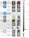
Extended Data Fig. 1 ∣. Pipeline procedures.

a–f, Summary of procedures involved in each step of the pipeline. g, Rig for parallel recording from six Neuropixels probes. Scale bar, 10 cm. h, Example retinotopic map used for targeting probes to six cortical visual areas. Scale bar, 1 mm. i, Image of Neuropixels probes during an experiment, with area boundaries from h overlaid in orange. Probe tips are marked with white dots. Scale bar, 1 mm. j, Box plot of the number of units recorded per area per experiment, after filtering based on ISI violations (<0.5), amplitude cutoff (<0.1) and presence ratio (>0.95) (see Methods and Extended Data Fig. 4 for quality metric definitions and distributions). Box plot edges represent upper and lower quartiles; centre line represents the median; whiskers represent 5th to 95th percentile range; open circles represent any data points beyond the edge of the whiskers. k, Histogram of the number of simultaneously recorded cortical and thalamic visual areas per experiment (n = 58 experiments).

Extended Data Fig. 2 ∣. Pipeline quality control.

a–f, Major quality control metrics for each pipeline step, with examples of passing and failing experiments. The number of mice failing quality control at each stage is shown on the right.

Extended Data Fig. 3 ∣. Data processing steps.

a, Data from the Neuropixels probe is split at the hardware level into two separate streams for each electrode: spike band and LFP band. b, The spike band passes through offset subtraction, median subtraction and whitening steps before sorting. The resulting data can be viewed as an image, with dimensions of time and channels, and colours corresponding to voltage levels. c, The LFP data are down sampled to 1.25 kHz and 40 μm channel spacing before packaging. d, We use the Kilosort2 to match spike templates to the raw data. The output of this algorithm can be used to reconstruct the original data using information about template shape, times and amplitudes. e, The spike and LFP data are packaged into Neurodata Without Borders (NWB) 2.0 files. f, The outputs of Kilosort2 are passed through a semi-automated quality control procedure to remove units with artefactual waveforms. Only units with obvious spike-like characteristics are used for further analysis.

Extended Data Fig. 4 ∣. Unit quality metrics.

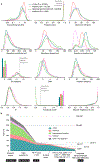
a, Density functions for twelve quality control metrics, plotted for units in cortex, hippocampus, thalamus and midbrain, aggregated across experiments. Default AllenSDK thresholds are shown as dotted lines. b, Unit selection flowchart for generating manuscript figures. Note that we do not use the default AllenSDK filters in this work, but instead use a receptive field P value of 0.01 as the primary metric for selecting units for analysis. CCFv3 structure labels used for region identification are as follows: cortex (VISp, VISl, VISrl, VISam, VISpm, VISal, VISmma, VISmmp, VISli, VIS), thalamus (LGd, LD, LP, VPM, TH, MGm, MGv, MGd, PO, LGv, VL, VPL, POL, Eth, PoT, PP, PIL, IntG, IGL, SGN, VPL, PF, RT), hippocampal formation (CA1, CA2, CA3, DG, SUB, POST, PRE, ProS, HPF), midbrain (MB, SCig, SCiw, SCsg, SCzo, SCop, PPT, APN, NOT, MRN, OP, LT, RPF), other/nonregistered (CP, ZI, grey).

Extended Data Fig. 5 ∣. Aligning units with the Common Coordinate Framework (CCFv3).

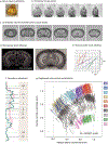
a, After each experiment, the brain is removed and cleared using a variant of the iDISCO method. b, The cleared brain is imaged at 400 rotational angles using a custom-built optical projection tomography microscope. c, We generated an isotropic 3D volume from rotational images using a computational tomography algorithm. d, Key points from the CCFv3 template brain are manually identified in each individual brain. e, Points along each fluorescently labelled probe track are manually identified in the volume. Using the key points from d, we define a warping function to translate points along the probe axis into the Common Coordinate Framework. f, We then align the regional boundaries to boundaries in the physiological data, primarily the decrease in unit density at the border between the cortex and hippocampus, and between the hippocampus and thalamus. The shaded area represents unit density on each recording site, and pink dots represent low-frequency LFP power (<10 Hz) along the probe axis. g, Finally, units in the database are mapped to a 3D location in the CCFv3 and are assigned a structure label. Units in cortex are also assigned a relative depth (0, surface; 1, white matter) and a layer label (L1, L2/3, L4, L5 or L6), on the basis of the annotation of the CCFv3 template volume (10-μm resolution).

Extended Data Fig. 6 ∣. Details of the visual stimulus set and receptive field mapping procedure.

a, Example frames from each type of stimulus. Green arrows indicate direction of motion. The natural scene image is shown illustrative purposes. The natural scene images shown to the mice are from refs. and . b, Timing diagram for visual stimulus set #1, known as ‘Brain Observatory 1.1’. c, Timing diagram for visual stimulus set #2, known as ‘Functional Connectivity’. d, Receptive field mapping used 20° diameter drifting gratings flashed for 250 ms in each of 81 randomized locations on the screen. A spike raster for one unit shows the timing of spikes on each of 45 trials with the stimulus at a particular location. Collapsing over trials yields a peristimulus time histogram for each location. Collapsing over time yields a spike count for each spatial bin. A matrix of spike counts represents the receptive field for this unit. e, To calculate receptive field properties, the receptive field is first smoothed with a Gaussian filter, and all pixels above a threshold value are selected. The centre of mass of the above-threshold pixels indicates the receptive field location, while the total number of above-threshold pixels indicates the area. These processing steps are shown for 25 receptive fields randomly chosen from one experiment.

Extended Data Fig. 7 ∣. Functional connections between visual cortical areas.

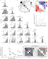
a, Peak offset distributions aggregated across 25 mice for each area combination, during drifting gratings presentation. The total number of pairs (n) is labelled in each sub-panel. Dashed black line indicates zero time lag. Dashed red line indicates the median of the distribution. b, Fraction of within- and between-area unit pairs exhibiting sharp peaks, out of all simultaneously recorded pairs. c, Combined median of peak offsets across mice (averaged across mice; n = 25 mice in total) for each pair of cortical areas. d, Correlation between the median peak offset and the difference in hierarchy scores among 21 pairs (lower triangle and diagonal of the matrix). e, Relationship between average 3D Euclidean distance between units simultaneously recorded in each pair of areas (following registration to the CCFv3) and their hierarchy score difference. r_P, Pearson correlation coefficient; r_S, Spearman’s rank correlation coefficient. f, Average number of sharp peak connections per mouse for jitter-corrected CCGs calculated during spontaneous activity (30 min grey screen period). Pixels masked with grey indicate no sharp peaks were detected. g, Average directionality score across mice during spontaneous activity.

Extended Data Fig. 8 ∣. Simulation of functional connectivity profiles for different network structures.

a, Directionality score (DS) and total hierarchy score calculated from actual data. Left, an example distribution of peak offsets between V1 (source) and LM (target); middle, DS matrix for all area combinations; right, mean DS for each source area to all target areas, which gradually decreases along the hierarchy. The maximum difference of the mean DS across areas represents the total hierarchy score for the real network. b–f, Simulations based on different hypothetical network structures. Because the standard deviation of peak offset distribution in our measured CCG time lag distribution is 3.7 ± 0.2 ms and the median CCG time lag of neighbouring areas is 1.1 ± 0.4 ms, we simulated Gaussian distributions of the model peak offsets with σ = 4 and μ = 1 for neighbouring hierarchical levels (μ = L_i − L_j between hierarchical levels i and j). See Methods for additional details of this simulation. b, A fully recurrent network where all nodes (areas) are at the same hierarchical level and have unbiased reciprocal connections (μ = 0). c, A two-level, one-to-all network that models parallel feedforward projections from V1, with all other areas recurrently connected with one another in an unbiased way. d, A three-level network, assuming V1 at the lowest level, RL, LM and AL at the second level, AM and PM at the top level. e, A six-level hierarchical network with each area at a distinct hierarchical level. Network parameters were constrained by real data (σ = 4 and μ = 1 for neighbouring hierarchical levels, and μ = L_i − L_j between any hierarchical levels i and j). f, A six-level hierarchical network with a narrow distribution of peak offsets (σ = 1) that simulates a paucity of feedback connections.

Extended Data Fig. 9 ∣. Statistics and additional analysis of hierarchy measures.

a, P values for pairwise comparisons of time to first spike between areas (two-sided Wilcoxon rank–sum test with Benjamini-Hochberg false discovery rate correction). b, Comparison between time-to-first-spike measured in response to the onset of the flash stimulus (‘flash’) versus during the inter-stimulus interval which corresponds to spontaneous firing (‘spontaneous’). The colour scheme is the same as in Fig. 4; error bars represent mean ± 95% confidence intervals; n = 15,713 units from 58 mice. c, Relationship between time-to-first spike and mean firing rate for a given area, either in response to the flash stimulus, or during the inter-trial interval (‘spontaneous’). d, P values for pairwise comparisons of receptive field size between areas. Colour scale is the same as in a. e, P values for pairwise comparisons of modulation index between area. Colour scale is the same as in a. f, Distribution of intrinsic timescale across units in each of 8 areas. g, Correlation between mean intrinsic timescale and anatomical hierarchy score. The absence of a significant correlation is inconsistent with the findings from ref. , in which it was shown that intrinsic timescale increases with hierarchical level in primates. This discrepancy may stem from differences between mouse and primate neocortex, or the fact that the areas we have recorded do not span the full range of the mouse cortical hierarchy. In addition, it is known that standard exponential fitting procedures produce biased and unreliable timescale estimates, which may account for the null result we observed. h, P-values for pairwise comparisons of response decay timescales between areas. Colour scale is the same as in a. i, Distribution of overall firing rates for all units in each area. j, Correlation between mean firing rate and anatomical hierarchy score. k, Relationship between change modulation index and anatomical hierarchy score, grouped by hit and miss trials. l, Relationship between pre-change response and anatomical hierarchy score, grouped by active and passive trials. m, Relationship between change response and anatomical hierarchy score, grouped by active and passive trials. n, Relationship between baseline firing rate and anatomical hierarchy score, grouped by active and passive trials. o, Decoder accuracy as a function of number of neurons used for decoding, averaged across all brain regions and behaviour sessions. p, Decoder accuracy for each brain region (mean ± s.e.m., averaged across sessions) is not correlated with the anatomical hierarchy score. r_P, Pearson correlation coefficient; r_S, Spearman’s rank correlation coefficient.

Extended Data Fig. 10 ∣. Layer-wise analysis.

a, Distribution of unit depths by area. 0 = surface, 1 = white matter. Normalized depth is measured along lines normal to the cortical surface (‘cortical streamlines’), rather than distance along the probe. b, Time-to-first-spike, receptive field area, modulation index, and response decay timescale analysed separately for each cortical layer. Colours are the same as those used in Fig. 4. Error bars represent mean ± 95% bootstrap confidence intervals. On average, in comparison to deep layers (5 and 6), superficial layers (2/3 and 4) had an earlier time to first spike (2.59 ms difference, P = 2.7 × 10⁻¹⁹, two-sided Wilcoxon rank-sum test), smaller receptive fields (109° difference, P = 1.1 × 10⁻³³), higher modulation index (0.09 MI difference, P = 5.0 × 10⁻²³), and faster response decay timescale (6.6 ms difference, P = 3.8 × 10⁻³³). The presence of slightly earlier spikes in L2/3 than L4 of V1 is probably due to the existence of direct connections from LGN to L2/3 of this area. r_P, Pearson correlation coefficient; r_S, Spearman’s rank correlation coefficient. c, Average number of sharp peak pairs for each area and layer combination. Units in each area are bi-partitioned into superficial (layers 2–4) and deep layers (layers 5–6). d, Directionality score (averaged across mice) as an indicator of feedforward and feedback asymmetry. Areas ordered by hierarchy and layers arranged from superficial to deep. e, Directionality score based on average within-layer and between-layer distributions in d; superficial layers tend to drive deep layers within a cortical area.

Fig. 1 ∣. A standardized pipeline for electrophysiology in the mouse visual system.

a, Data collection pipeline, with the average age of mice (in days) indicated below. b, Schematic of probe insertion trajectories through visual cortical (V1, LM, AL, RL, AM, PM) and thalamic (LGN, LP) areas. c, Example raster plot of 405 simultaneously recorded units from 8 visual areas during drifting grating stimuli (15 Hz, 2 Hz or 4 Hz), with hippocampal (HPC) local field potential, mouse running speed and pupil diameter shown below. d, Raster plots of spike times for different drifting grating stimuli from an exemplar V1 unit. Single-trial responses are represented by a star plot (right), in which stimulus orientation and temporal frequency are indicated by angle and radius, respectively, and firing rate is indicated by the intensity of the pink blob. e, Raster plots and peri-stimulus time histograms of the full-field flash stimulus, for the same unit as in d. f, Raster plot of spike times for 81 conditions of the Gabor stimulus for the same unit. Summing the spike counts across 45 trials at each location produces a spatial receptive field, shown on the right. Spike count is quantified over a 250-ms window. g, Mean fraction of units with significant receptive field across eight visual areas, with hippocampus included as a control (see Methods). Data are mean ± s.d., and dots show the results of individual sessions.

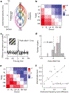
Fig. 2 ∣. Functional connectivity recapitulates the anatomical hierarchy.

a, Anatomical hierarchy scores of the eight areas of Interest recomputed from ref. . b, Replotting the anatomical hierarchy scores from a, showing the difference in score between all cortical areas. All areas have significantly different anatomical hierarchy scores, except for RL and LM (Wilcoxon rank-sum test, P = 0.08; see Methods). c, An example cross-area ‘sharp peak’ spiking interaction between a pair of units in V1 and LM. d, Distribution of CCG peak time lags between V1 and LM in one example mouse. The median (3.9 ms) is shown by the red line. e, Directionality scores calculated from peak offset distributions across 25 mice for each pair of cortical areas. Statistical testing (two-sided Wilcoxon rank-sum test) revealed that the peak offset distributions of neighbouring areas were significantly different from within-area distributions, except for AL–PM (P = 0.08). f, Correlation between directionality score and anatomical hierarchy score difference (n = 21 pairs; lower triangle and diagonal of the matrices in b and e), indicating a link between structure and function. r_P, Pearson correlation coefficient.

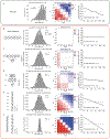
Fig. 3 ∣. Four measures of hierarchical processing applied to the mouse visual system.

a, Mean response (baseline-subtracted) to a full-field flash stimulus for units in eight visual regions. b, Distribution of time to first spike in response to the flash stimulus across all units in each of eight areas. c, Correlation between mean time to first spike and hierarchy score obtained from anatomical tracing studies. d, Outlines of the extent of the mean receptive field for each area, at 50% of the peak firing rate. Example mean receptive fields for the LGN and the AM are shown on the left. e, Distribution of receptive field sizes across all units. f, Correlation between mean receptive field size and anatomical hierarchy score. g, Raster plots showing the response of exemplar LGN and AM units to a 2-Hz drifting grating stimulus, with corresponding modulation index (MI). h, Distribution of modulation index across all units. i, Correlation between mean modulation index and anatomical hierarchy score. j, Mean autocorrelation averaged across all units in each area in the 250-ms period following the onset of a full-field flash stimulus. k, Distribution of response decay timescales across all units in each area. l, Correlation between mean response decay timescales and anatomical hierarchy score; n = 7,837 units from 58 mice. m, Key indicating the colour code used in the graphs, the number of units per area and the total number of mice per area. See Extended Data Fig. 4b for unit selection criteria. Data are mean ± 95% bootstrap confidence intervals. n = 15,713 units from 58 mice unless otherwise specified.r_S, Spearman correlation coefficient.

Fig. 4 ∣. Higher-order areas signal behaviourally relevant changes in image identity more strongly than lower-order areas.

a, Experimental setup for the active (left) and passive (right) change detection tasks. b, After training, mice had high hit and low false alarm rates, with an average d′ of 2.0 ± 0.1 (n = 12 mice, 21 sessions). c, Raster plots of exemplar units from the LGN, V1 and AM before and after change (n = 50 trials). d, Population response averaged over all units in the LGN, V1 and AM. For each area, the response to the change and pre-change image is shown as a darker and lighter line, respectively. The line represents the mean and the shaded areas represent s.e.m. e, Correlation between mean time to first spike after image change and anatomical hierarchy score across all eight areas; data are mean ± 95% bootstrap confidence intervals. f, Correlation between mean change modulation index and anatomical hierarchy score across all eight areas. Closed circles indicate responses during active behaviour, and open circles indicate responses during passive stimulus replay; data are mean ± 95% bootstrap confidence intervals. g, Schematic of random forest decoding analysis to identify change versus non-change trials, and comparison with mouse behaviour. h, Pearson correlation of decoder prediction (change probability) and mouse behavioural response (hit/miss) across trials. Data are mean ± s.e.m. across sessions; see Methods for details of included units. i, Key indicating the colour code used in the graphs in e, f and h, the number of units per area and the total number of mice per area. The natural scene images in a and g are shown for schematic purposes. The images shown to the mice are from refs. ^,.

References

1. Felleman DJ & Van Essen DC Distributed hierarchical processing in the primate cerebral cortex. Cereb. Cortex 1, 1–47 (1991). - PubMed
1. de Vries SEJ et al. A large-scale standardized physiological survey reveals functional organization of the mouse visual cortex. Nat. Neurosci 23, 138–151 (2020). - PMC - PubMed
1. Harris JA et al. Hierarchical organization of cortical and thalamic connectivity. Nature 575, 195–202 (2019). - PMC - PubMed
1. Carandini M et al. Do we know what the early visual system does? J. Neurosci 25, 10577–10597 (2005). - PMC - PubMed
1. Olshausen BA & Field DJ How close are we to understanding V1? Neural Comput. 17, 1665–1699 (2005). - PubMed
Publication types
LinkOut - more resources