SERENA: Particle Instrument Suite for Determining the Sun-Mercury Interaction from BepiColombo

Abstract

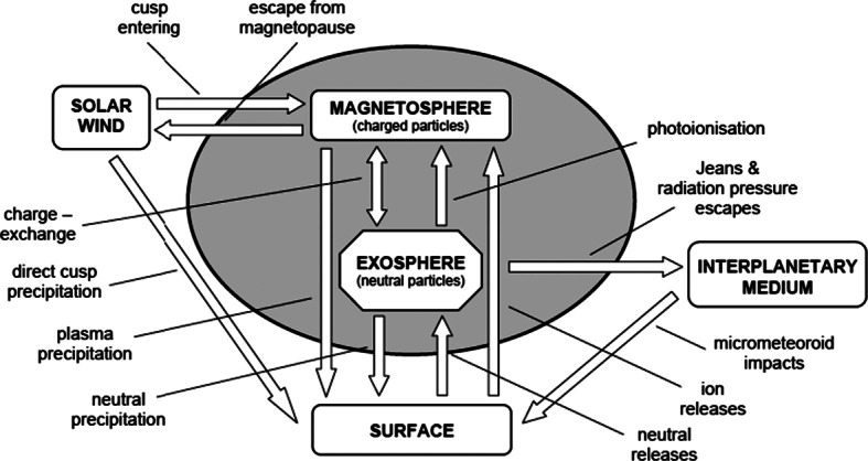
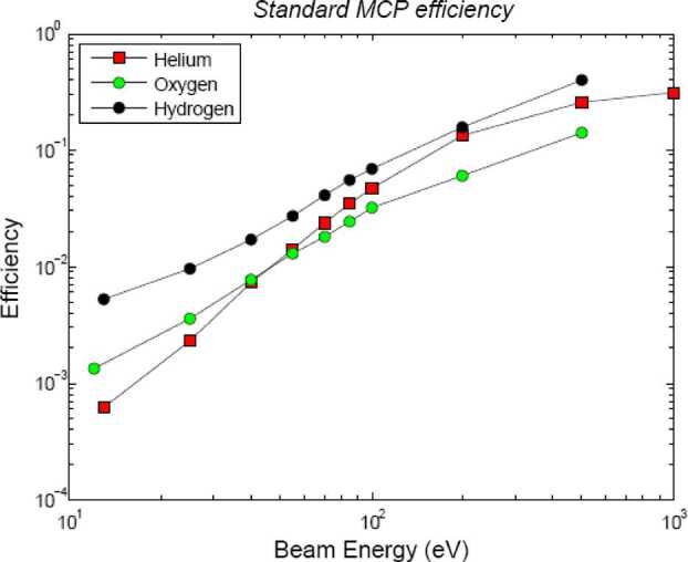
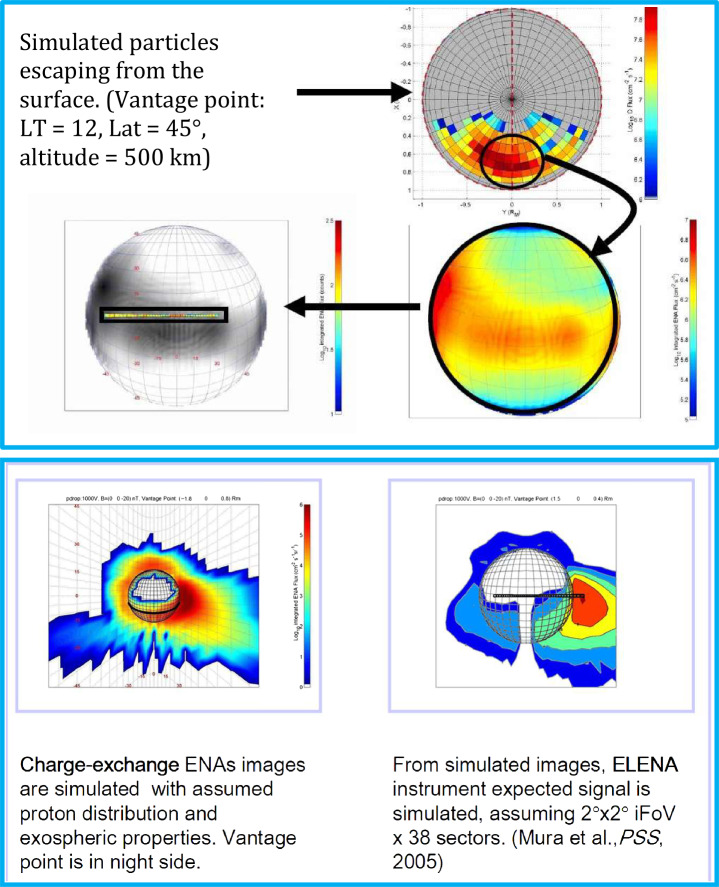
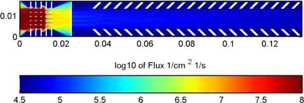
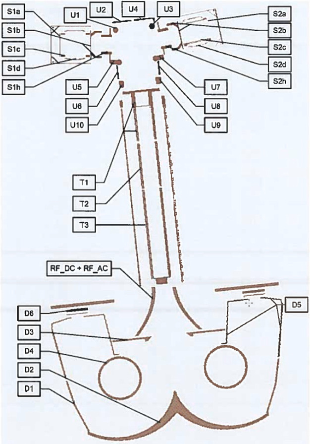
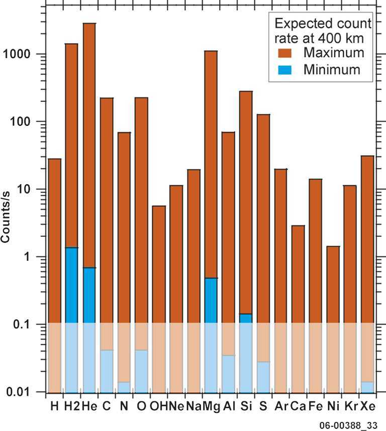
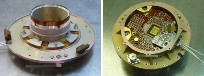
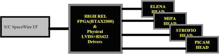
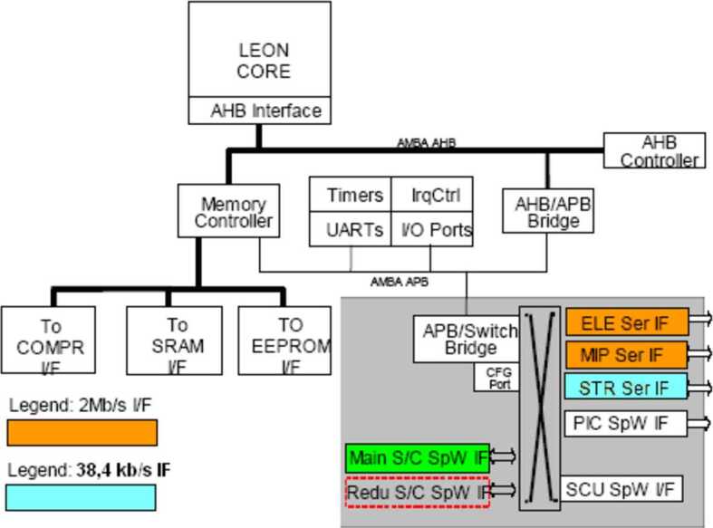
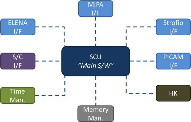
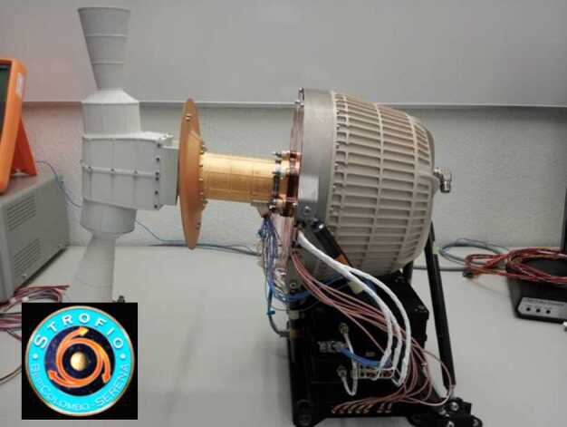
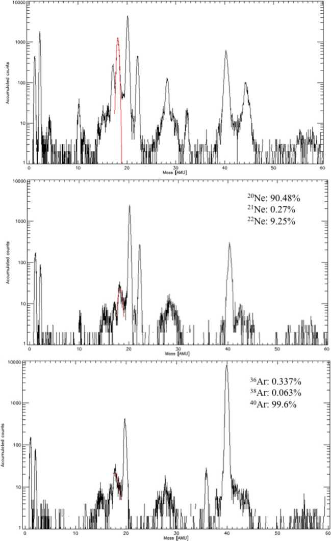
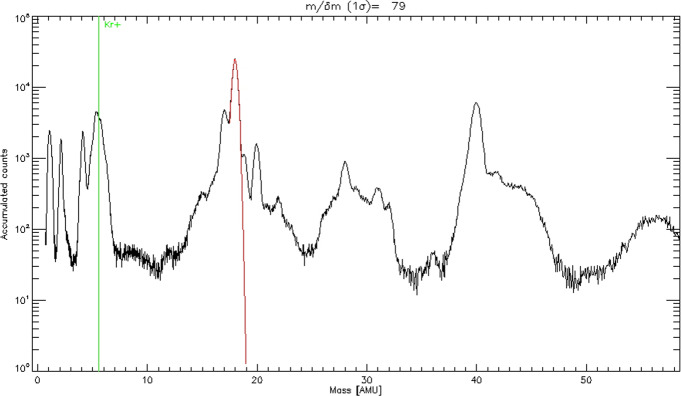
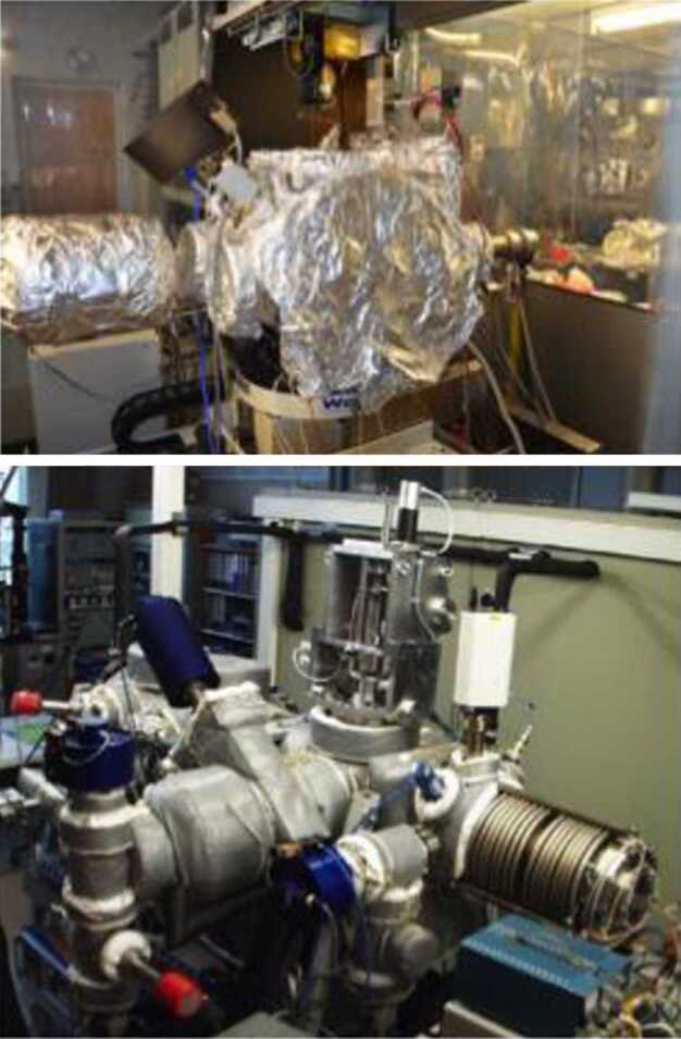
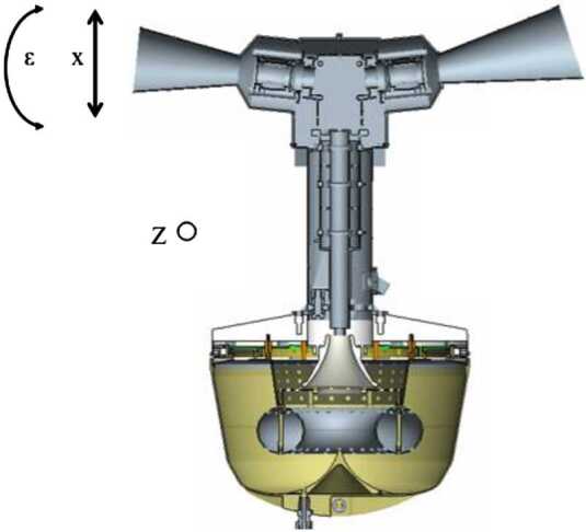
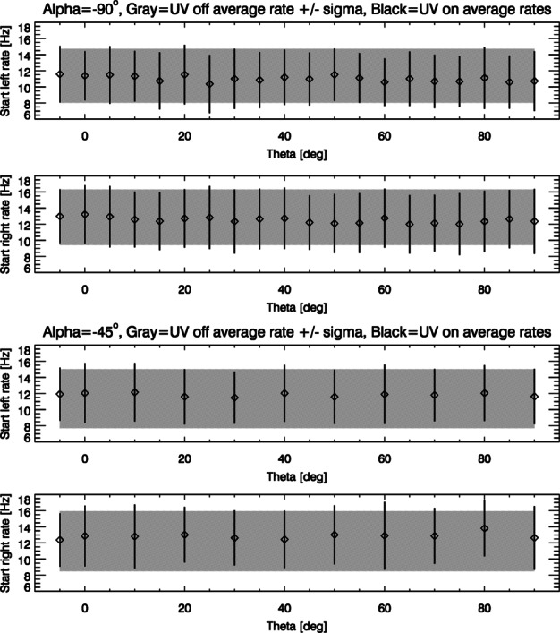
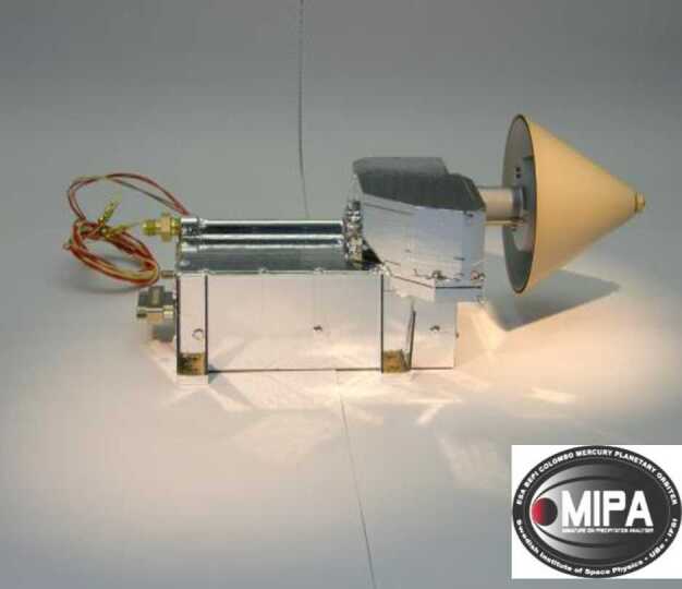
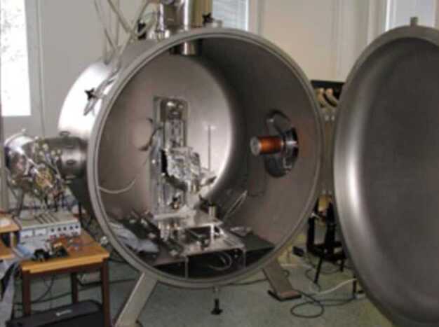
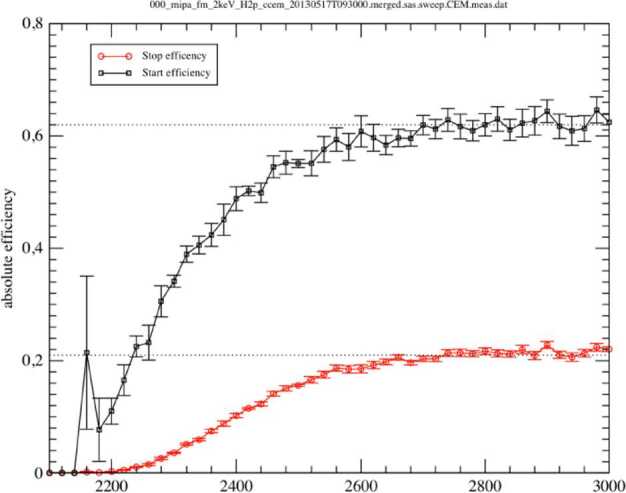
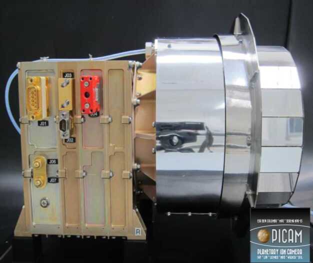
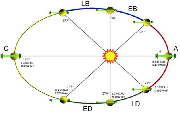
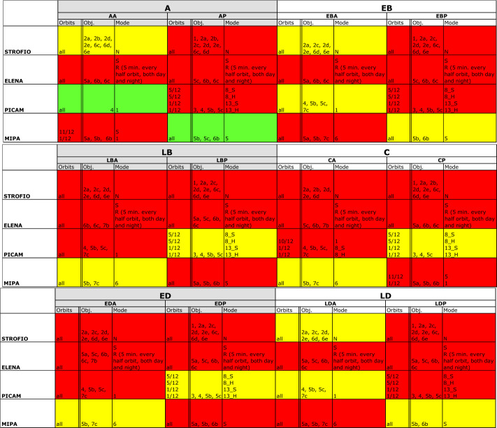
The ESA-JAXA BepiColombo mission to Mercury will provide simultaneous measurements from two spacecraft, offering an unprecedented opportunity to investigate magnetospheric and exospheric particle dynamics at Mercury as well as their interactions with solar wind, solar radiation, and interplanetary dust. The particle instrument suite SERENA (Search for Exospheric Refilling and Emitted Natural Abundances) is flying in space on-board the BepiColombo Mercury Planetary Orbiter (MPO) and is the only instrument for ion and neutral particle detection aboard the MPO. It comprises four independent sensors: ELENA for neutral particle flow detection, Strofio for neutral gas detection, PICAM for planetary ions observations, and MIPA, mostly for solar wind ion measurements. SERENA is managed by a System Control Unit located inside the ELENA box. In the present paper the scientific goals of this suite are described, and then the four units are detailed, as well as their major features and calibration results. Finally, the SERENA operational activities are shown during the orbital path around Mercury, with also some reference to the activities planned during the long cruise phase.

Keywords: BepiColombo space mission; Mercury’s environment; Particle instrumentation.

Fig. 1

Schematic of the interacting processes (from Milillo et al. 2005)

Fig. 2

‘Standard’ (1-h long) and ‘fixed-slit’ (time resolution about 4 m) images, during 7 June 2012. The black arrows approximately indicate the acquisition time of each image. In the lower part of each panel, the plots of the IMF values measured by MESSENGER are shown (Bx, By, Bz and |B|, see legend). The 1-hour averages are superposed to the 1-min plots (same colors) of each IMF components. The dashed areas mask the periods when the spacecraft was inside the Mercurian magnetosphere and no in situ IMF data are available (Massetti et al. 2017)

Fig. 3

Na D₂ emission intensity profile close to subsolar point observed at different Mercury’s year by MESSENGER/MASC (Cassidy et al. 2015)

Fig. 4

Na⁺-group (a), O⁺-group (b), and He⁺ (c) ion observed density along the MESSENGER orbit as a function of local time and planetary latitude (note that the northern data refer to lower altitudes). Observed regions with zero counts are colored black (Raines et al. 2015)

Fig. 5

Na ion distribution under the same southward IMF (B_Z = −5 nT) and SW conditions, subject to different assumptions of surface conductance. Upper panel: low conductivity; bottom panel: high conductivity. The resulting ion distributions are markedly different as the formation of an X-line further from the planet inhibits escape in the second case (Seki et al. 2013)

Fig. 6

Kinetic properties of protons and Na⁺-group ions within the cusp. Top panels (b), (e) are energy-resolved pitch angle distributions, which show the flow direction and energy of ions relative to the magnetic field in 20^∘ (protons) and 36^∘ (Na⁺-group) bins. Slices through these distributions in the parallel, anti-parallel and perpendicular directions are shown in the bottom panels (c), (f). The Figs show protons that are flowing down toward the surface, as well as loss cone of > 40^∘ in width. Low energy (100–300 eV) Na⁺-group ions appear to be upwelling from the surface, while those at energies up to 10 keV have large perpendicular energy components (Raines et al. 2014)

Fig. 7

Spacecraft potential for 5 electron temperatures as a function of plasma density, computed at 0.5 AU and 0.3 AU, by assuming a spherical body. The satellite photoelectron population is described by three Maxwellian distributions (energies: 1.5, 7.5 and 15 eV, and the saturation currents are 5 nA cm⁻² at 1 AU for 1.5 eV and 0.5 nA cm⁻² for the other two)

Fig. 8

Colour-coded precipitating (pitch angle < 90^∘, left panel) and the mirrored (pitch angle > 90^∘, right panel) proton flux in case of IMF (−20, 0, −5) nT at aphelion. Sample orbit of the MPO spacecraft (red line) and Mio (blue line) with magnetic field-lines are traced in the xz plane (Massetti private communication)

Fig. 9

Pitch angle H⁺ distribution at low- (left) and high-latitudes (right), computed in case of IMF (−20, 0, −5) nT at aphelion (Massetti private communications)

Fig. 10

Estimated size of the loss-cone (degrees) along possible MPO orbits. The x-axis shows the longitude (0^∘ towards the Sun) of the apogee. The $y$-axis shows the co-latitude of the true anomaly angle, apogee at 90^∘ and perigee at 270^∘

Fig. 11

Exospheres modelled for different surface release processes. (a) TD; (b) PSD; (c) ion-sputtering; (d) MIV (Mura et al. 2007)

Fig. 12

Chandrayaan-1 measurements taken shortly after the Moon crossed the Earth’s bow shock to the downstream direction. Energy spectra of the SW (right side, open squares) and of the corresponding reflected energetic hydrogen (left side, open circles) (Wieser et al. 2009)

Fig. 13

The energy distribution for sputtered particles, as a function of ejected Na and O particle energy in the case of 1 keV SW protons

Fig. 14

Estimated neutral back-scattered total flux impinging at the ELENA FOV sectors along the MPO day side orbit considering a yield of 10%

Fig. 15

Simulated ENA images, from a vantage point in the nightside (P1 = (1.8, 0, 0.8)RM) (left and middle panels) and at dawn sector (P2 = (0, 2.1, 0)RM) (right panel). Color is coded according to log (ENA flux), integrated over energy ranges: 100 eV–1 keV (left panel) and 1–10 keV middle panel, and 100 eV -10 keV right panel. The boundary conditions are: BIMF = (0, 0, −20) nT; PD = 10 kV (Mura et al. 2005)

Fig. 16

ELENA sensor concept

Fig. 17

MCP efficiency to H, He and O impact as a function of energy resulting from test performed by the IAPS team at the MEFISTO facility at the Bern University (Rispoli et al. 2013)

Fig. 18

Upper: Simulation of the energy-integrated (between 20-1000 eV) signal from vantage point MLT=1200, 45^∘ elevation and 500 km altitude is shown in the upper panel. The horizon at in this position is zoomed in the bottom-right panel and the slice of ELENA FOV is evidenced in the bottom-left panel. Bottom: Energy-integrated H ENA from the night side apoherm (left panel). The instantaneous FOV of the linear array of the ELENA sensor is shown as a slice in the right panel (from Mura et al. 2005, 2006)

Fig. 19

Ion flux at the instrument entrance suppressed by the −1000 V/+1000 V charge stopping deflectors

Fig. 20

Simion Model of Strofio, showing the 30 different electrodes, whose voltages were determined and optimized during the calibration activities

Fig. 21

Expected Strofio performance at Mercury. Both elements and isotopes will be resolved in Mercury’s exosphere

Fig. 22

Strofio’s count rates at 400 km altitude, estimated from Table 1. Background is estimated at the 0.1 count/s level

Fig. 23

Mass spectrum of H₂, He, Ne, N₂, Ar, O₂, CO₂

Fig. 24

MIPA model with aperture top hat

Fig. 25

Min pitch-angle covered by MIPA as a function of the beta-angle and true anomaly angle. $(0,0)$ corresponds to the noon-midnight orbit with the pericenter at the subsolar point

Fig. 26

Max pitch-angle covered by MIPA as a function of the beta-angle and true anomaly angle. $(0,0)$ corresponds to the noon-midnight orbit with the pericenter at the subsolar point

Fig. 27

The pitch-angle range covered by MIPA as a function of the beta-angle and true anomaly angle. $(0,0)$ corresponds to the noon-midnight orbit with the pericenter at the subsolar point

Fig. 28

Field of view of MIPA (red line). The colour scale (in arbitrary units where highest value corresponds to 100% transparency) shows a pixel example

Fig. 29

Simulation of primary pixels of the MIPA instrument for one of three rotationally symmetric sections of the instrument

Fig. 30

Comparison between laboratory results (left) and simulations for the field of view of one MIPA pixel. The right hand panel shows a photo of the instrument

Fig. 31

Sketch of the PICAM instrument

Fig. 32

Sketch of PICAM ion trajectories

Fig. 33

Annular array of blades of the inner part of mirror M1

Fig. 34

Electrostatic Analyser ESA, consisting of three parts, which are screwed together

Fig. 35

M2 serving as a convex lens to map the ions onto the detector

Fig. 36

Gating electrodes for TOF measurements

Fig. 37

Detector block diagram

Fig. 38

Pixel geometry and mapping of the collector

Fig. 39

detector top and bottom view with Electronics

Fig. 40

SCU Architecture

Fig. 41

Instrument physical data communication diagram

Fig. 42

The Main SCU S/W functionalities diagram

Fig. 43

SCU S/W transition mode diagram

Fig. 44

ELENA Proto-Flight Model (PFM)

Fig. 45

ELENA internal design. The red-circles highlight the external and internal charge particle-deflectors

Fig. 46

Counts vs PP applied. FS test: 1-keV (above left) and 3-keV (above right) H⁺ 4-keV O⁺ (below left). PFM test. PFM test: 1-keV H⁺ (below right)

Fig. 47

1-keV O angular scan vs acquisition number (left), T_int=10 s. The sector distribution of the scanning as a function of incidence angle (right) shows the angle-sector correspondence and spread. Note that the efficiency is lower at higher angle as shown by the normalization factor (below)

Fig. 48

(left) Normalized angular scan counts for 1-keV H⁺. (right) Observed sector normalization factors for 1-keV O (blue line), and theoretical curve of the normalization factor (dashed black line)

Fig. 49

Expected counts at 0^∘ angle to the normal for different flux intensities, energies, species and charges vs real counts at the peak sector. Comparison with the 1 by 1 curve (dashed line)

Fig. 50

Counts/s of UV at ELENA when a source of intensity 1.5 10¹¹ ph/(cm² s) at -40^∘ (above), 0^∘ (middle) and 30^∘ (below) has been used, T_int=10 s

Fig. 51

Strofio Flight Model/FM)

Fig. 52

Relationship between count rate and ionization current at a pressure of 1.08×10⁻⁷ mbar

Fig. 53

Multiple pressure scans

Fig. 54

Relation between countrate vs Pressure × Current

Fig. 55

Top: Strofio mass resolution without a velocity filter. Middle: mass resolution of Ne isotopes with a velocity filter. Down: mass resolution of Ar isotopes with a velocity filter

Fig. 56

Strofio mass range for two turns

Fig. 57

Photo of CASYMIR and the beam facility at the University of Bern calibration facility

Fig. 58

Scan directions with respect to Strofio FOV

Fig. 59

Angular acceptance and response in the $\epsilon$ direction

Fig. 60

Mass composition of rest gas around Rosetta

Fig. 61

(a) Input H₂O distributions; blue: from spacecraft; red: from Mercury. (b) End-to-end transmission using a velocity filter

Fig. 62

Velocity filter effects on Strofio response for (a) Ar and H₂O, (b) Ne and H${}_2\text{O}$

Fig. 63

Results of UV contamination tests for Strofio MCPs

Fig. 64

MIPA Flight model

Fig. 65

IRF-Kiruna calibration facility

Fig. 66

Detector efficiencies as a function of the applied voltages

Fig. 67

Dependence of the STOP efficiency on the count rate

Fig. 68

MIPA ESA energy response

Fig. 69

The ESA voltage as a function of the beam energy to establish the analyser constant

Fig. 70

TOF spectrum for ions with M/q = 1, 2, 3, 14

Fig. 71

MIPA angular sectors scheme. Note that the Zenith direction is D0 = ${180}^{\circ }\times {90}^{\circ }$ with $\mathrm{\Delta }\alpha ={30}^{\circ }\times {20}^{\circ }$)

Fig. 72

(left) MIPA calibration with 2 keV N⁺ in the Zenith direction (D0 sector). (right) Full coverage at 2 keV N⁺. From BC-SRN-TR-40020-01-00 _MIPA FM Calibration Report

Fig. 73

(left) MIPA calibration with 9 keV N⁺ in D0 sector. (right) Full coverage at 9 keV N⁺. From BC-SRN-TR-40020-01-00 _MIPA FM Calibration Report

Fig. 74

(left) MIPA calibration with 500 eV N⁺ in D0 sector. (right) Full coverage at 500 eV N⁺. From BC-SRN-TR-40020-01-00 _MIPA FM Calibration Report

Fig. 75

MIPA calibration with 2 keV N⁺ in D12-1 sector. From BC-SRN-TR-40020-01-00 _MIPA FM Calibration Report

Fig. 76

Placement of MIPA pixels based on detailed calibration data processing

Fig. 77

PICAM Flight Model

Fig. 78

Line plots for each PICAM ring and their elevation peak values (Nominal elevations are 15^∘ to 75^∘ from ring 5 to 1)

Fig. 79

Panel (a) shows the azimuth and elevation mapping of the incoming ion beam (He⁺, 500 eV) entering the centre of sector 4 (azimuth=210^∘ elevation=65^∘). Panel (b) and (c): The best fitting of the ion beam pattern, resolved by numerical calculations. Panel b represents the actual number of counts from each pixel, when the particles are landing on the detector as shown in panel (c)

Fig. 80

Count rates obtained with the flight model versus M1 voltage for different directions of the incoming ion beam (upper panel: He+ at 200 and 1000 eV, respectively; lower panel: N2+ at 500 eV). The half width $\mathrm{\Delta }$E1/2 of the energy distribution for each scan is shown

Fig. 81

ToF spectra in single pulse mode for two different species (He⁺, ${\text{N}}_2^{+}$) obtained at 500 (upper panels) and 1000 eV (lower panel)

Fig. 82

ToF spectra in Hadamard mode for 500 (N2+, He+, first and second panel) and 1000 (He+, third panel) eV ions measured with the flight model

Fig. 83

Transparency (fraction of registered to incoming ion flux) for several sectors as a function of elevation angle with the flight model

Fig. 84

SCU Mode Transition Diagram

Fig. 85

ELENA Mode Transition Diagram

Fig. 86

Strofio State Diagram

Fig. 87

Strofio Mode Transition Diagram

Fig. 88

MIPA Mode Transition Diagram realized by SW resident on SCU

Fig. 89

MIPA Low level Sensor Mode

Fig. 90

PICAM Mode Transition Diagram

Fig. 91

SERENA Science Operations Scenario

Fig. 92

SERENA science goals and their priority per orbit phase and instrument. Red: high priority, Yellow: normal priority. Green: low priority

References

1. Anderson B.J., Johnson C.L., Korth H., Purucker M.E., Winslow R.M., Slavin J.A., Solomon S.C., McNutt R.L., Jr., Raines J.M., Zurbuchen T.H. Science. 2011;333:1859–1862. doi: 10.1126/science.1211001. - DOI - PubMed
1. Balsiger H., Altwegg K., Bertaux J.-L., Bochsler P., Carignan G.R., Eberhardt P., Fisk L.A., Fuselier S.A., Ghielmetti A.G., Gliem F., Gombosi T.I., Kopp E., Korth A., Livi S., Mazelle C., Young D.T. Rosetta Orbiter Spectrometer for Ion and Neutral Analysis—ROSINA. Adv. Space Res. 1998;21(11):1527.
1. Balsiger H., Altwegg K., Bochsler P., Eberhardt P., Fischer J., Graf S., Jäckel A., Kopp E., Langer U., Mildner M., Müller J., Riesen T., Rubin M., Scherer S., Wurz P., Wüthrich S., Arijs E., Delanoye S., De Keyser J., Neefs E., Nevejans D., Rème H., Aoustin C., Mazelle C., Médale J.-L., Sauvaud J.A., Berthelier J.-J., Bertaux J.-L., Duvet L., Illiano J.-M., Fuselier S.A., Ghielmetti A.G., Magoncelli T., Shelley E.G., Korth A., Heerlein K., Lauche H., Livi S., Loose A., Mall U., Wilken B., Gliem F., Fiethe B., Gombosi T.I., Block B., Carignan G.R., Fisk L.A., Waite J.H., Young D.T., Wollnik H. ROSINA - Rosetta Orbiter Spectrometer for Ion and Neutral Analysis. Space Sci. Rev. 2007;128:745–801.
1. J. Benkhoff, G. Murakami, W. Baumjohann, S. Besse, E. Bunce, M. Casale, G. Cremosese, K.-H. Glassmeier, H. Hayakawa, D. Heyner, H. Hiesinger, J. Huovelin, H. Hussmann, V. Iafolla, L. Iess, Y. Kasaba, M. Kobayashi, A. Milillo, I.G. Mitrofanov, E. Montagnon, M. Novara, S. Orsini, E. Quemerais, U. Reininghaus, Y. Saito, F. Santoli, D. Stramaccioni, O. Sutherland, N. Thomas, I. Yoshikawa, J. Zender, BepiColombo – mission overview and science goals. Space Sci. Rev. (2020, submitted)
1. Berezhnoy A. Chemistry of impact events on Mercury. Icarus. 2018;300:210–222.
LinkOut - more resources