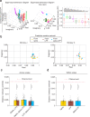
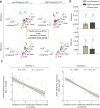
. 2021 Jan 27;12(1):607.
doi: 10.1038/s41467-020-20197-x.

Multiscale low-dimensional motor cortical state dynamics predict naturalistic reach-and-grasp behavior

Affiliations

Multiscale low-dimensional motor cortical state dynamics predict naturalistic reach-and-grasp behavior

Hamidreza Abbaspourazad et al. Nat Commun. .

Abstract

Motor function depends on neural dynamics spanning multiple spatiotemporal scales of population activity, from spiking of neurons to larger-scale local field potentials (LFP). How multiple scales of low-dimensional population dynamics are related in control of movements remains unknown. Multiscale neural dynamics are especially important to study in naturalistic reach-and-grasp movements, which are relatively under-explored. We learn novel multiscale dynamical models for spike-LFP network activity in monkeys performing naturalistic reach-and-grasps. We show low-dimensional dynamics of spiking and LFP activity exhibited several principal modes, each with a unique decay-frequency characteristic. One principal mode dominantly predicted movements. Despite distinct principal modes existing at the two scales, this predictive mode was multiscale and shared between scales, and was shared across sessions and monkeys, yet did not simply replicate behavioral modes. Further, this multiscale mode's decay-frequency explained behavior. We propose that multiscale, low-dimensional motor cortical state dynamics reflect the neural control of naturalistic reach-and-grasp behaviors.


Conflict of interest statement

The authors declare no competing interests.

Figures

Fig. 1
Fig. 1. Task set-up and recording regions for two non-human primates (Monkey J and Monkey C).
a Both subjects performed a 3D naturalistic reach-and-grasp task in a 50 cm × 50 cm × 50 cm workspace. An object located on a wand was always present in the 3D workspace and visible to the monkey. The wand was continuously moved by the experimenter to random locations spanning a large spatial area in front of the subjects. Subjects naturalistically reached to the object (without a go cue), grasped it, and then returned to the resting position. They performed the reach-and-grasp continuously in time for the whole course of the recording session (without a trial structure). There was no go cue, no instructions as to when to reach, and no requirements on reach, hold and grasp durations as the subjects performed the task. Subjects performed reaches to the objects, decided on the hold durations, reach durations, and grasp durations naturalistically. We used motion capture technology using retroreflective markers to track 27 (Monkey J) or 25 (Monkey C) joint angles on the right shoulder, elbow, wrist, and fingers at each point in time. The picture is recreated from marker trajectories of a sample recording session for Monkey J. b Recording regions covered primary motor cortex (M1), dorsal premotor cortex (PMd), ventral premotor cortex (PMv), and prefrontal cortex (PFC) for Monkey J and covered PMd and PMv for Monkey C. Recording electrodes are shown as black circles. Brain sulci (PS principal sulcus, AS accurate sulcus, CS central sulcus, PD precentral dimple) around the recording regions are shown by grey lines. The inter-electrode distance was 1.5 mm.
Fig. 2
Fig. 2. Multiscale dynamical modeling and modal analysis.
a We first learn the dynamical model from the neural activity in the training set. The neural activity can be in the form of spiking, LFP, or combined spike-LFP activity. b After learning the dynamical model, we find the principal modes that characterize neural dynamics. Each principal mode has a unique pair of dynamical characteristics consisting of a decay and frequency and indicating how fast one component of neural response decays in time and with what frequency it rings over time in response to excitations. c To get the principal modes, for the same neural activity, we learn dynamical models of various latent state dimensions. For each dimension, we indicate the location of the modes corresponding to their real and imaginary values on a plane parallel to the xy plane and intersecting the z axis at that dimension. We finally cluster the modes using K-means clustering to find the vertical clusters, each corresponding to a different location on the xy plane and thus different decay-frequency characteristics. d In the test set, we use the learned dynamical model to estimate the modes and states. We then use the estimated state to predict behavior and predict neural activity one-step-ahead into the future, and we separate the contribution of each mode in these predictions. By comparing the contribution of each mode with true behavior and neural activity, we get each modes’ behavior prediction accuracy and one-step-ahead prediction accuracy of neural activity. This accuracy is quantified with correlation coefficient (CC) for behavior and LFP features and with prediction power (PP) for spike events (Methods).
Fig. 3
Fig. 3. Both spiking and LFP network activity exhibit several principal modes in their dynamics.
a Eigenvalue-dimension diagram for spiking (top) and LFP (bottom) network activity in one sample session. The vertical clusters are principal modes each shown with a different color. Modes that cannot be categorized in clusters are shown in grey. b The top view of eigenvalue-dimension diagram in a. For simplicity, in this view we show the modes for dimensions higher than 10. c The top view of eigenvalue-dimension diagram in (b) in the interpretable decay-frequency domain (Methods). NP and ND represent non-periodic or non-decaying dynamics, respectively. d Principal modes that form vertical clusters exist in every session. Each data point (grey dot) represents the mean distance of the members in one vertical mode cluster in one session from its centroid in the x–y plane. Data points are shown for all clusters in all sessions. Bars represent the mean over data points and error bars represent the 95% confidence bounds of this mean. A principal mode cluster must have a mean member distance to cluster centroid that is significantly smaller than half of chance-level distance (P < 1.6 × 10−4, Ns = 39, 17 (top) and Ns = 53, 31 (bottom) mode clusters across sessions in Monkey J and C, one-sided Wilcoxon signed-rank test, FDR-corrected) (Methods). Asterisks indicate significance of this comparison (*P < 0.05, **P < 0.005, and ***P < 0.0005). Source data are provided as a Source Data file.
Fig. 4
Fig. 4. In both spiking and LFP activity, one mode is dominantly predictive of behavior.
a Joint angle prediction accuracy statistics are shown for the members of the mode clusters in spiking network activity in the sample session shown in Fig. 3. Colors represent the colored clusters in Fig. 3. The yellow cluster termed predictive mode has significantly higher prediction accuracy than every other cluster (P < 8.1 × 10−28, Ns > 97 yellow cluster members, one-sided Wilcoxon rank sum test). The line inside boxes shows median, box edges represent the 25th and 75th percentiles, whiskers show the minimum and maximum values excluding outliers and red crosses indicate the outliers. Outliers are the points that are >1.5 times the box size away from the beginning and end of the box. b Similar to (a) for LFP network activity, where the brown cluster (predictive mode) has significantly higher prediction accuracy than every other cluster (P < 1.4 × 10−4, Ns > 99 brown cluster members, one-sided Wilcoxon rank sum test). c In each monkey, among all principal modes in spiking activity, the prediction accuracy of one of them (termed predictive mode) is significantly better than that of the second best principal mode shown by black box plots (yellow vs. black). The same result holds for LFP activity, and its predictive mode and second best principal mode (brown vs. black). Significance is shown by asterisks (P < 1.8 × 10−20, Ns = 35 and 20 cross-validation folds for Monkeys J and C, one-sided Wilcoxon signed-rank test). d Boxplot of the prediction power (PP) of mode clusters in predicting spiking activity. Higher prediction power indicates better one-step-ahead prediction of spiking activity. The same predictive mode that dominantly predicted behavior had the best one-step-ahead prediction of spiking activity (yellow mode cluster, P < 9.9 ×  10−17, Ns > 97 cluster members, one-sided Wilcoxon rank sum test). e Similar to (d) but for the correlation coefficient (CC) of mode clusters in one-step-ahead prediction of LFP. The same predictive mode cluster that dominantly predicted behavior had the best one-step-ahead prediction of LFP activity (brown mode cluster, P < 3.5 × 10−11, Ns > 99 cluster members, one-sided Wilcoxon rank sum test). Source data are provided as a Source Data file.
Fig. 5
Fig. 5. The predictive mode is multiscale, i.e., is shared across scales of brain activity.
a Eigenvalue-dimension diagram for combined spike-LFP activity. Figure convention is the same as Figs. 3 and 4. Combined spike-LFP network activity also exhibited several principal modes among which again one (cyan) was dominantly predictive of behavior (P < 3.4 × 10−12, Ns > 125 cyan cluster members, one-sided Wilcoxon rank sum test). Boxplot outliers are a small fraction of data and mainly correspond to learned mode members at low dimensions when mode estimation has not converged yet. b The predictive modes across sessions in the two monkeys. Each dot represents the centroid of the predictive mode cluster in one experimental session for spiking (yellow), LFP (brown) and combined spike-LFP (cyan) network activity. c The location of the predictive mode was similar across scales of activity. The distance between the predictive mode centroids across scales, pooled across monkeys and experimental sessions was significantly smaller than chance-level (P < 6.8 × 10−22, Ns = 121 possible pairwise distances across scales, one-sided Wilcoxon signed-rank test). Each bar represents the mean of all possible pairwise distances between cluster centroids across scales shown in (b). For example, yellow-brown bar represents the mean of all pairwise distances between any yellow and brown dot in (b). Grey dots show all pairwise distances. Error bars show 95% confidence bound of the mean. Asterisks show the significance of comparison with chance-level distance with a similar convention as in Fig. 3. d The location of the predictive mode was similar across monkeys and experimental sessions (P < 5.7 × 10⁻¹¹, Ns = 55 possible pairwise distances within scales, one-sided Wilcoxon signed-rank test). Same as (c) but for pairwise distances between cluster centroids within scales in (b). For example, yellow bar represents the mean of all pairwise distances between any two yellow dots in (b). Source data are provided as a Source Data file.
Fig. 6
Fig. 6. Distance to the multiscale predictive mode explains behavior prediction accuracy.
a For both monkeys, using the combined spike-LFP activity improved the estimation of the multiscale predictive mode across channel sets (Methods). The distance of the estimated modes to the multiscale predictive mode significantly decreased when using spike-LFP activity in combination compared with separately. Each channel set used a baseline of random five LFP or spike single-scale channels and then added random 25 spike or LFP channels to them, respectively. The location of the multiscale predictive mode was defined as the average of the single-scale predictive modes estimated using all channels to get the best estimate (average of brown and yellow dots in Fig. 5b). b For both monkeys, there was a positive correlation between the reduction in distance and improvement in joint angle prediction accuracy in CC (P < 1.5 × 10−5, Ns = 1400 and 800 Monte Carlo samples in Monkey J and C, two-sided corrected resampled paired t test). Each dot represents one cross-validation fold from one channel set. To show the results across sessions, values are z scored for each session. R represents the Pearson’s correlation coefficient and P its p value corrected by the resampled t test (see Methods). Black line is the linear least-square fit representing the mean prediction accuracy for different distances and the shaded area is the 95% confidence bound of the mean. Source data are provided as a Source Data file.
Fig. 7
Fig. 7. The multiscale predictive mode was present in both low-frequency and high-frequency bands of LFP activity.
a For a sample experimental session (top: Monkey J, bottom: Monkey C), the top view of the eigenvalue-dimension diagram is shown for low-frequency (theta + alpha + beta; left) and high-frequency (gamma; right) bands of LFP activity. The yellow circle is the average location of the predictive mode clusters in the spiking network activity in Fig. 5b, which we used as the ground-truth location of the multiscale predictive mode in this analysis. The members of the closest estimated principal mode cluster to the yellow dot are shown in orange. b In both monkeys and for both low-frequency and high-frequency bands of LFP activity, the mean distance of the closest estimated principal mode cluster to the multiscale predictive mode was significantly smaller than chance-level as shown by the asterisks with similar convention as in Fig. 3 (P < 6.4 × 10−5, Ns = 35 and 20 cross-validation folds across sessions for Monkeys J and C, FDR-corrected, one-sided Wilcoxon signed-rank test). The distance in each session is calculated between the centroid of the orange cluster and the yellow dot in (a). Bars represent mean across sessions and error bars are 95% confidence bound of the mean. c The distance of the estimated principal mode to the multiscale predictive mode is correlated with the behavior prediction accuracy for different frequency band combinations of LFP activity (theta + alpha, beta, gamma in addition to their pairwise combinations: theta + alpha + beta, theta + alpha + gamma and beta + gamma; P < 1.5 × 10−7, Ns = 42 and 24 frequency band combinations across sessions for Monkeys J and C, one-sided Wilcoxon signed-rank test, FDR-corrected). For each monkey, each dot represents one frequency band combination for one session. The distance and the prediction accuracy of the estimated principal mode in each session are z scored and then results are pooled across sessions. Similar to Fig. 6, black line is the linear least-square fit representing the mean prediction accuracy and the shaded area is the 95% confidence bound of the mean. Source data are provided as a Source Data file.
Fig. 8
Fig. 8. The multiscale predictive mode had a larger decay than other modes and both its decay and frequency explained naturalistic behavior prediction.
a Multiscale predictive modes in Fig. 5 had significantly larger decays than other complex-conjugate modes in spiking and LFP activity (P = 9.1 × 10−11, Ns > 22 spiking and LFP sessions, one-sided Wilcoxon rank sum test). Figure convention for boxplot and significance (asterisks) is similar to Figs. 3 and 4. Each grey dot shows the decay of one principal mode across subjects and experimental sessions. b Multivariate linear regression (MVLR) relating the principal mode’s prediction accuracy to its decay and frequency deviation. The deviations were computed as the mode’s decay and frequency absolute difference from those of the multiscale predictive mode (Methods). Both decay and frequency had significantly negative coefficient with p values reported by Pd and Pf, respectively (Ns = 66 complex-conjugate principal modes, two-sided paired t test). R2 shows the R-squared of the fitted MVLR model. Each green dot represents one complex-conjugate principal mode across subjects and experimental sessions. The black line shows the MVLR fitted line. c Perturbing decay (left) and frequency (right) of the multiscale predictive modes in the learned state-space model shows that both decay and frequency components explained naturalistic behavior prediction accuracy. Each dot represents the mean prediction accuracy of one perturbed mode across experimental sessions and monkeys; error bars represent 95% confidence bounds of the mean. The x axis is shown in log scale and represents the value of perturbed decay and frequency. Asterisks show whether the prediction of the perturbed mode is significantly different from that of the unperturbed multiscale predictive mode represented by a vertical dashed line, with conventions similar to Fig. 3 (n.s. is non-significant P > 0.05). Decays ~1−2 s had the best prediction accuracy (picked as the interval that had non-significant difference with the unperturbed mode, P = 4.1 × 10−2, Ns = 55 cross-validation folds, one-sided Wilcoxon signed-rank test, FDR-corrected). Also, mode frequencies ~0.17−0.3 Hz had the best prediction accuracy (picked as the interval that had non-significant difference compared with the unperturbed mode, P = 8.2 × 10−5, Ns = 55 cross-validation folds, one-sided Wilcoxon signed-rank test, FDR-corrected). Source data are provided as a Source Data file.

References

    1. Georgopoulos AP, Kalaska JF, Caminiti R, Massey JT. On the relations between the direction of two-dimensional arm movements and cell discharge in primate motor cortex. J. Neurosci. 1982;2:1527–1537. doi: 10.1523/JNEUROSCI.02-11-01527.1982. - DOI - PMC - PubMed
    1. Moran DW, Schwartz AB. Motor cortical representation of speed and direction during reaching. J. Neurophysiol. 1999;82:2676–2692. doi: 10.1152/jn.1999.82.5.2676. - DOI - PubMed
    1. Fetz EE. Are movement parameters recognizable coded in the activity of single neurons? Behav. Brain Sci. 1992;15:679–690.
    1. Reimer, J. & Hatsopoulos, N. G. The Problem of Parametric Neural Coding in the Motor System. Advances in Experimental Medicine and Biology. 629, 243–259 (Springer, Boston, MA, 2009). . - PMC - PubMed
    1. Yu BM, et al. Gaussian-process factor analysis for low-dimensional single-trial analysis of neural population activity. J. Neurophysiol. 2009;102:614–635. doi: 10.1152/jn.90941.2008. - DOI - PMC - PubMed

Publication types

LinkOut - more resources