. 2021 Feb;590(7845):344-350.
doi: 10.1038/s41586-020-03126-2. Epub 2021 Jan 27.

Integrated spatial genomics reveals global architecture of single nuclei

Affiliations

Integrated spatial genomics reveals global architecture of single nuclei

Yodai Takei et al. Nature. 2021 Feb.

Abstract

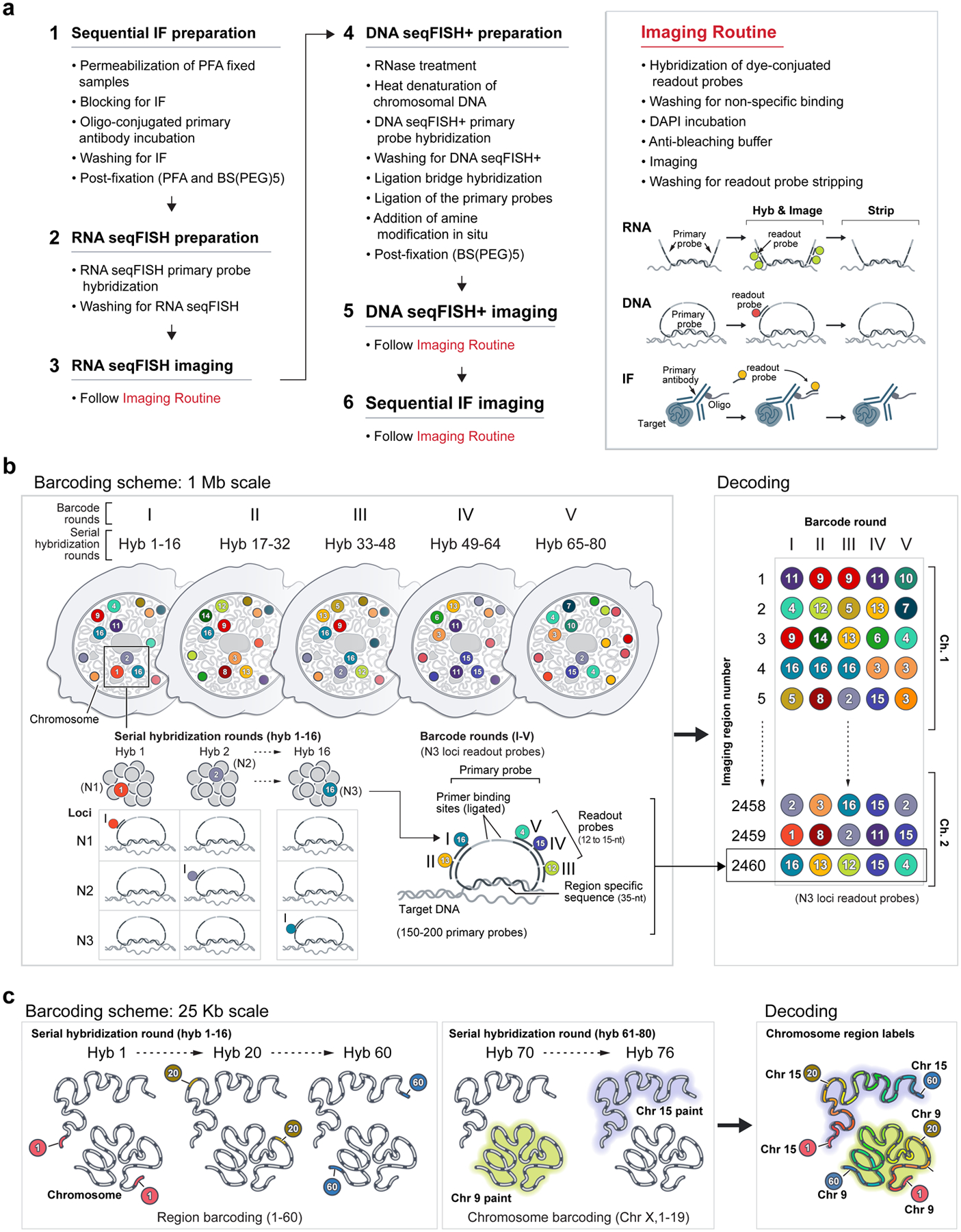
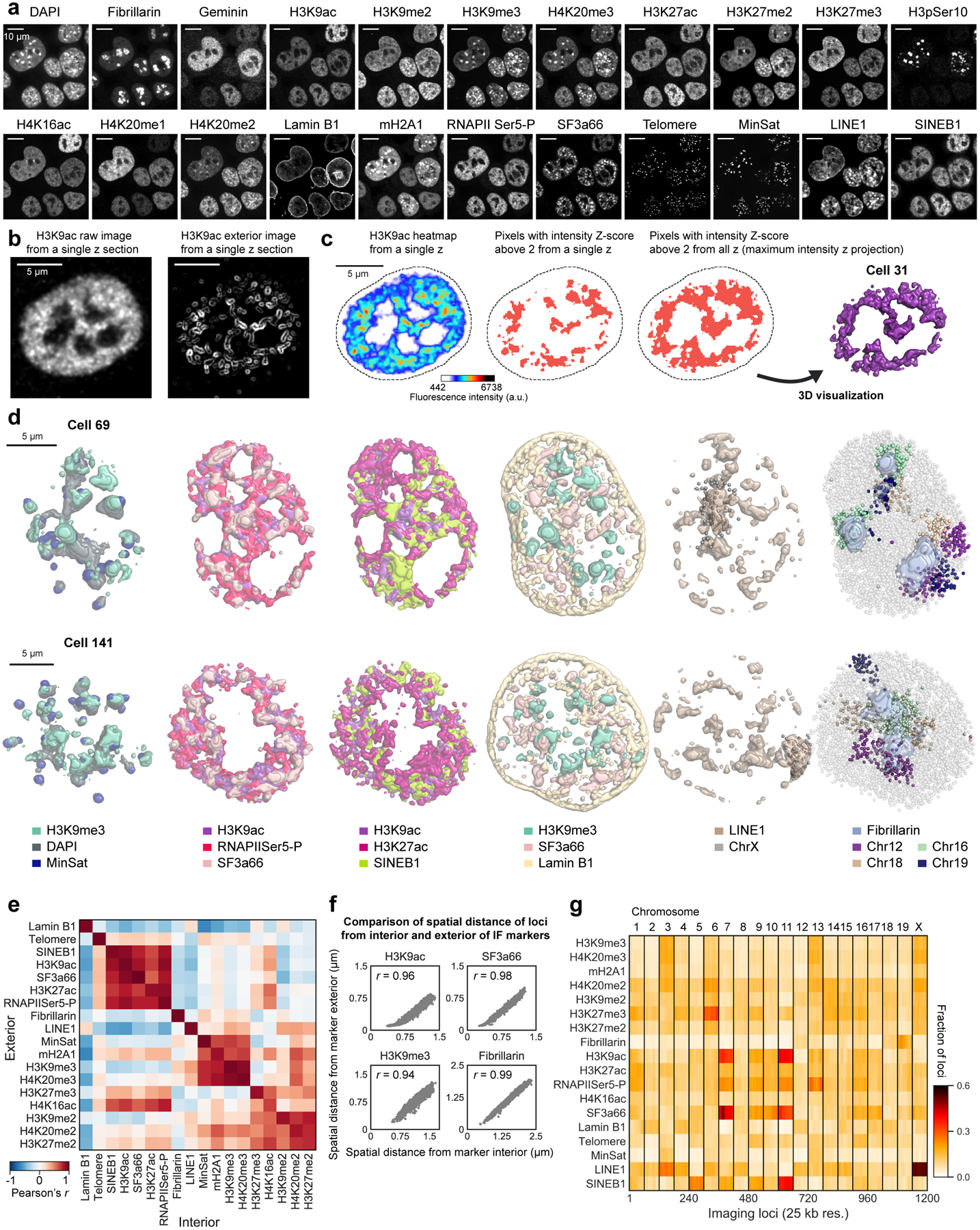
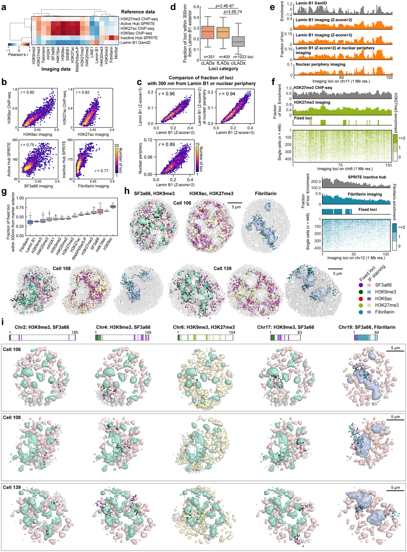
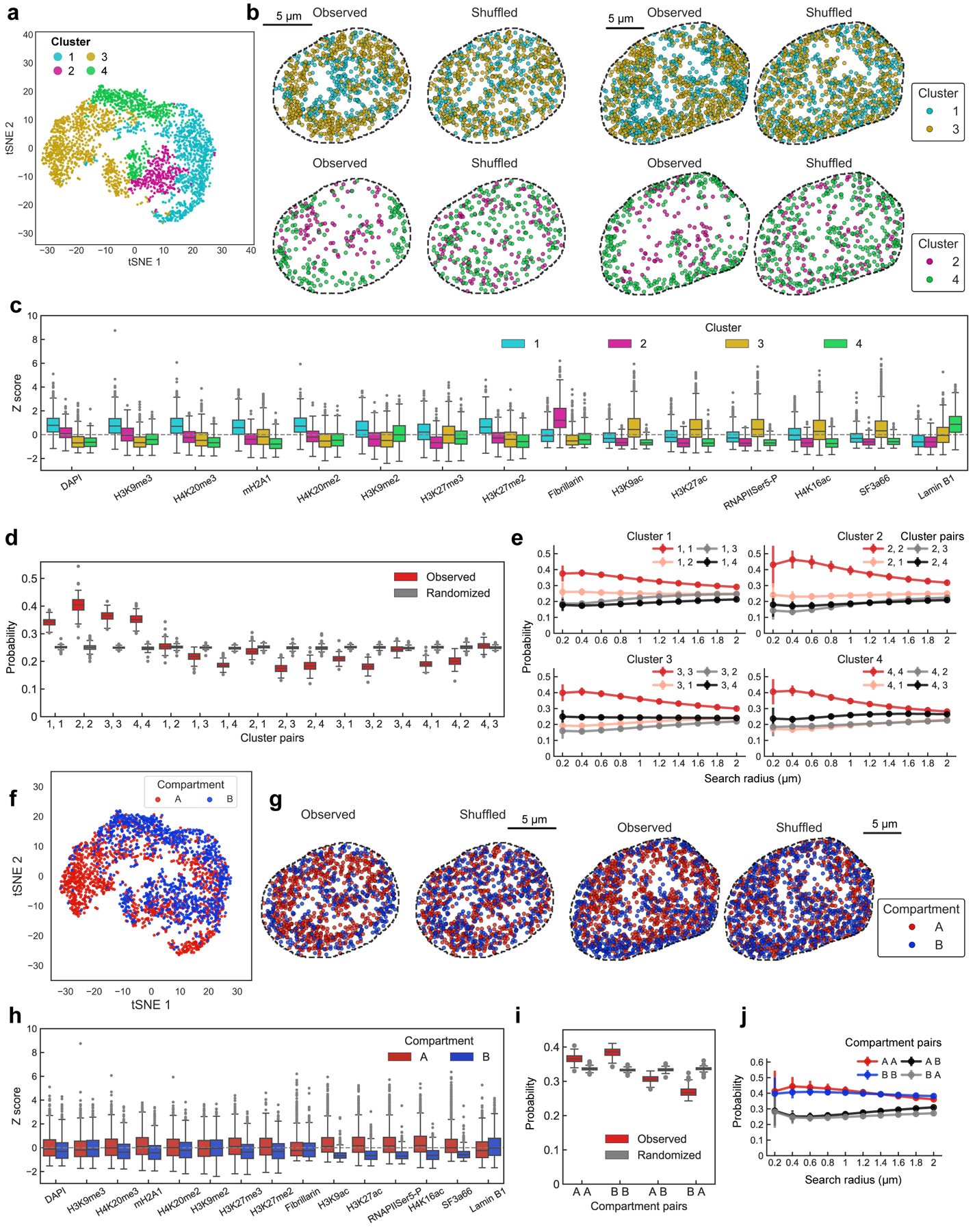
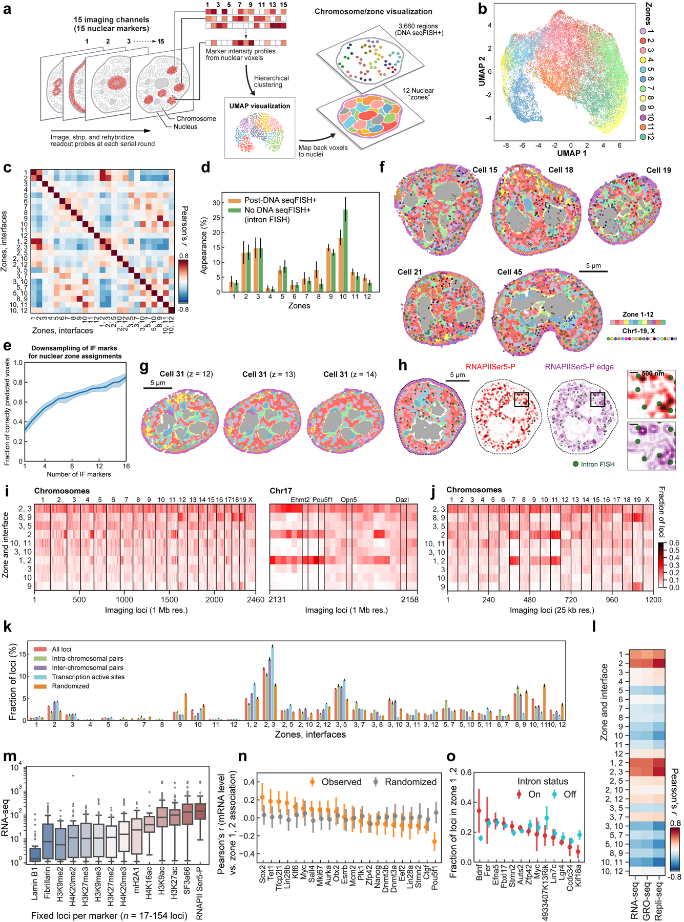
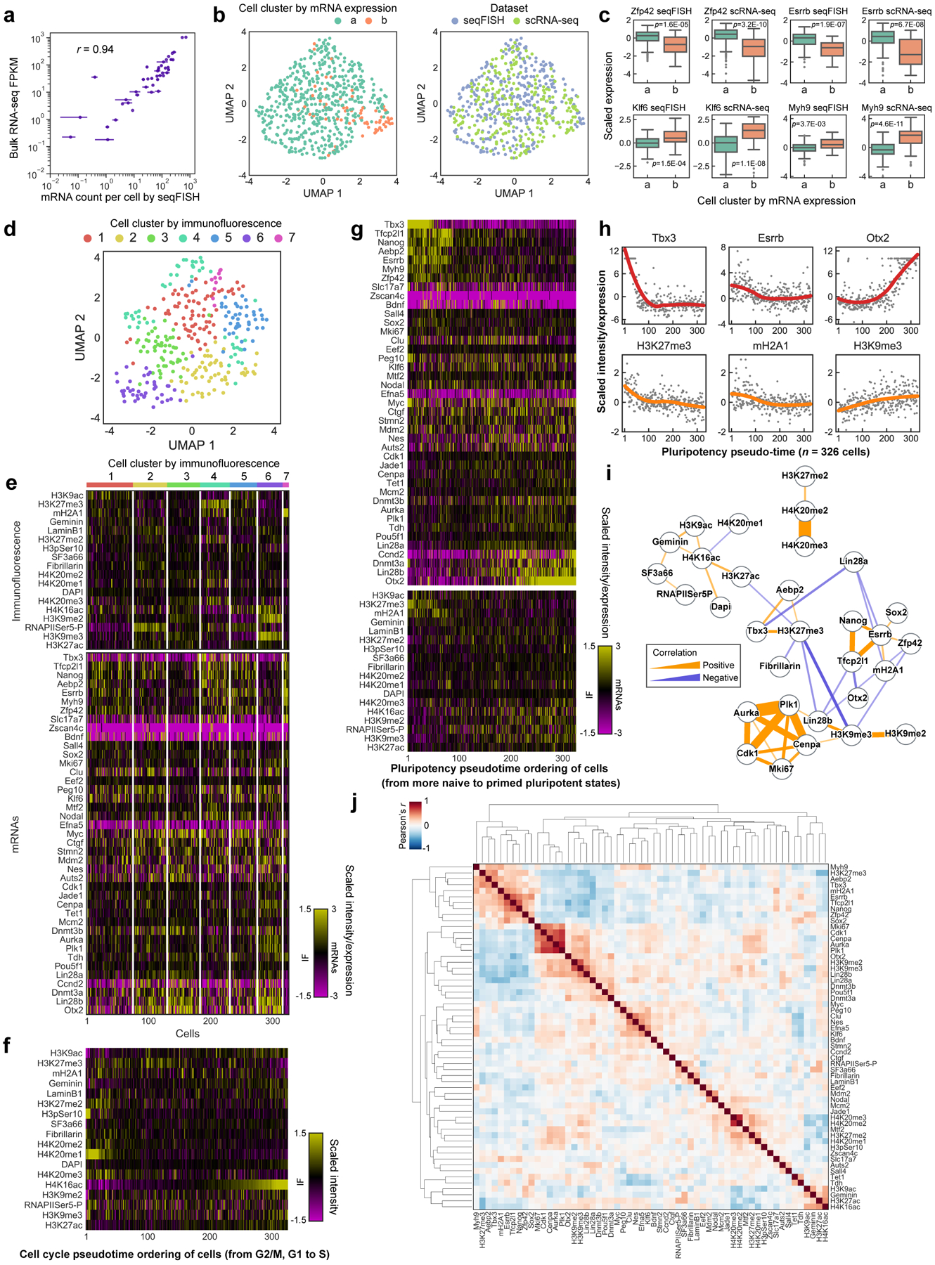
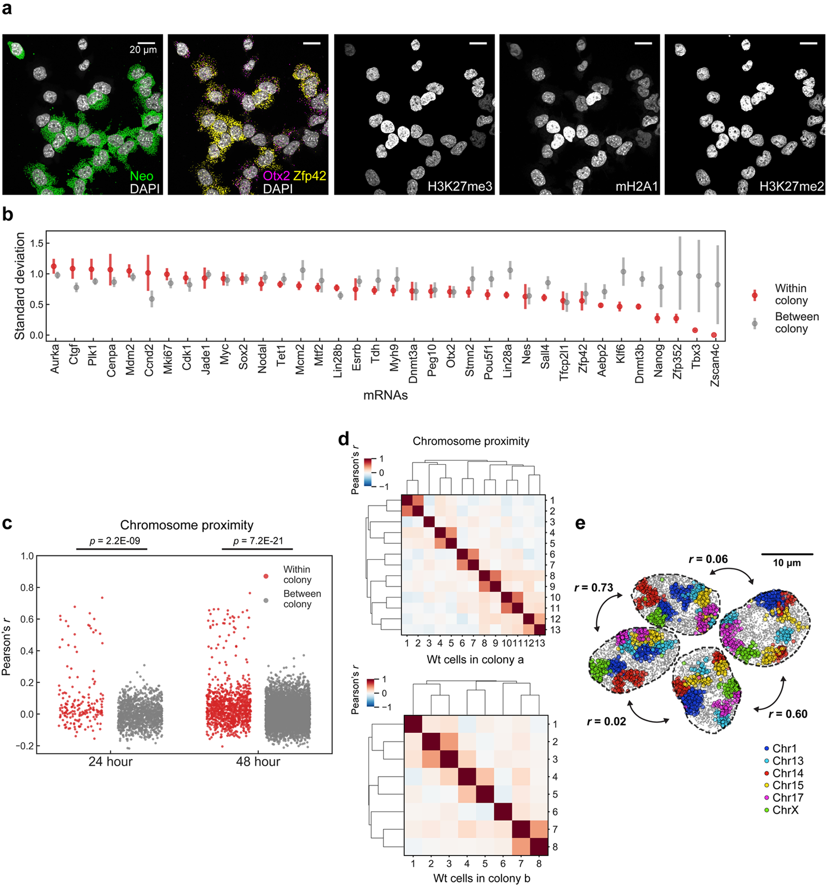
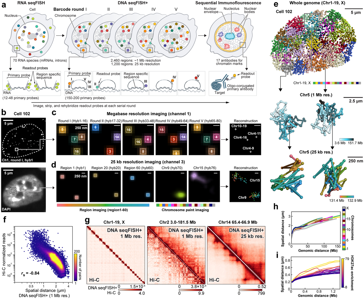
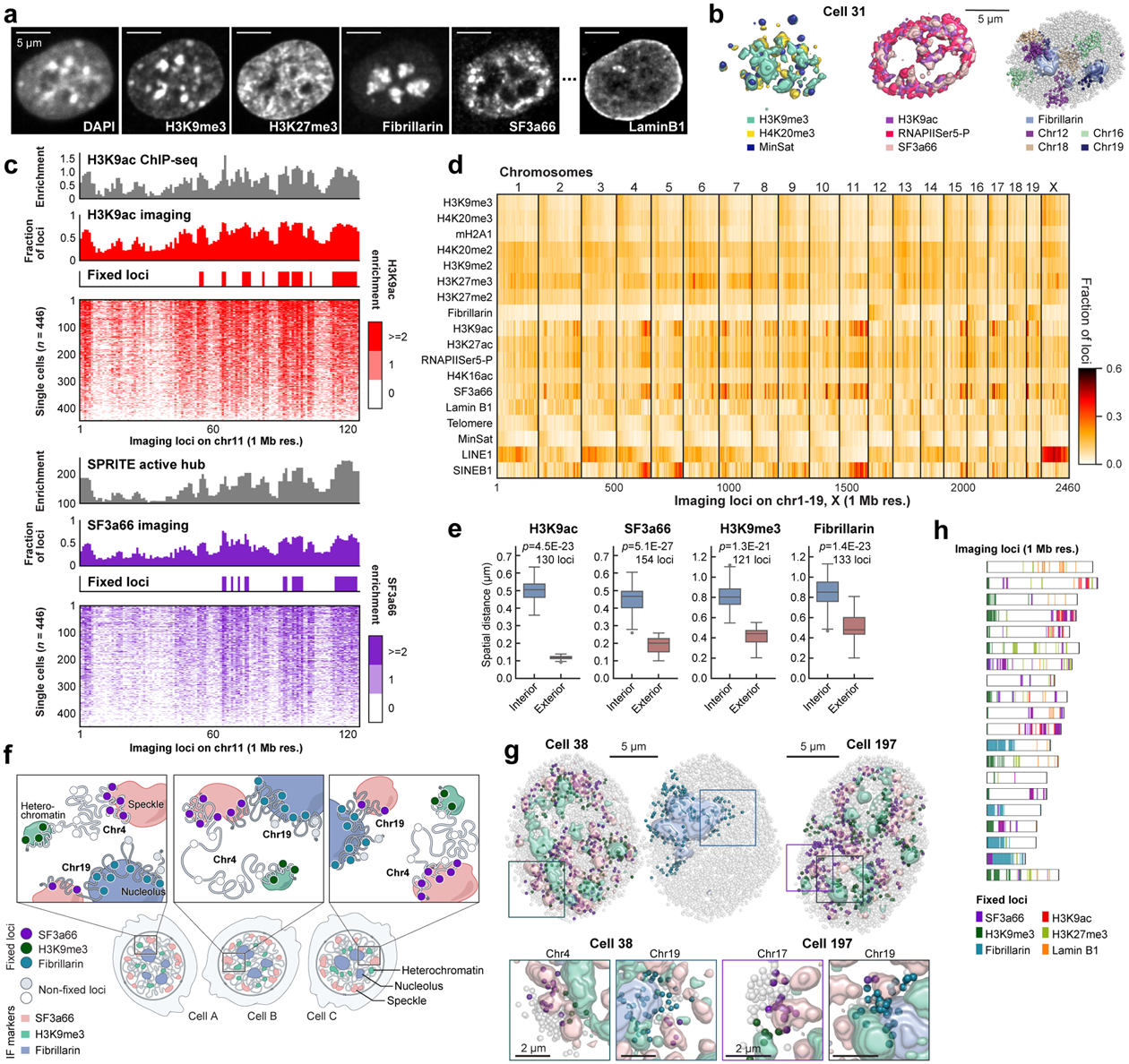
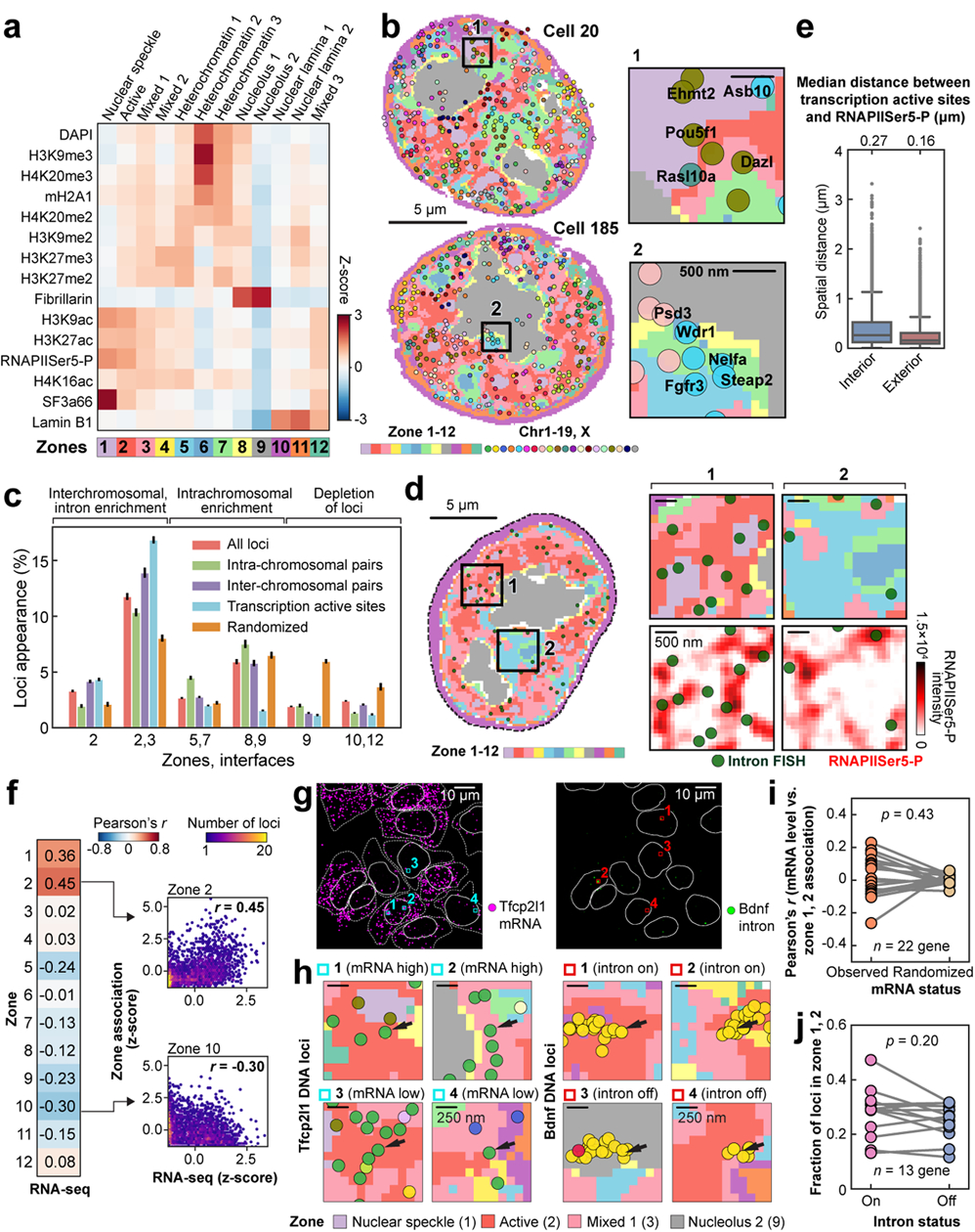
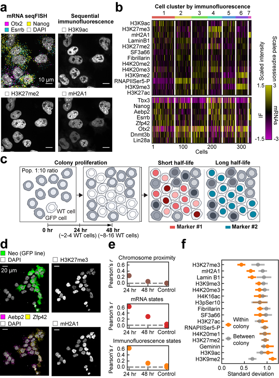
Identifying the relationships between chromosome structures, nuclear bodies, chromatin states and gene expression is an overarching goal of nuclear-organization studies1-4. Because individual cells appear to be highly variable at all these levels5, it is essential to map different modalities in the same cells. Here we report the imaging of 3,660 chromosomal loci in single mouse embryonic stem (ES) cells using DNA seqFISH+, along with 17 chromatin marks and subnuclear structures by sequential immunofluorescence and the expression profile of 70 RNAs. Many loci were invariably associated with immunofluorescence marks in single mouse ES cells. These loci form 'fixed points' in the nuclear organizations of single cells and often appear on the surfaces of nuclear bodies and zones defined by combinatorial chromatin marks. Furthermore, highly expressed genes appear to be pre-positioned to active nuclear zones, independent of bursting dynamics in single cells. Our analysis also uncovered several distinct mouse ES cell subpopulations with characteristic combinatorial chromatin states. Using clonal analysis, we show that the global levels of some chromatin marks, such as H3 trimethylation at lysine 27 (H3K27me3) and macroH2A1 (mH2A1), are heritable over at least 3-4 generations, whereas other marks fluctuate on a faster time scale. This seqFISH+-based spatial multimodal approach can be used to explore nuclear organization and cell states in diverse biological systems.


Conflict of interest statement

Competing Interest:

L.C. is a co-founder of Spatial Genomics Inc.

Figures

Extended Data Fig. 1 |
Extended Data Fig. 1 |. Detailed schematics of the integrated spatial genomics approach with DNA seqFISH+, RNA and intron seqFISH and multiplexed immunofluorescence.
a, Flow chart of the experimental procedures. Samples are fixed with PFA, followed by oligo-conjugated primary antibody incubation, post-fixation with PFA and BS(PEG)5, and RNA seqFISH. Then samples are prepared for DNA seqFISH+. This optimized protocol ensures good alignment between DNA seqFISH+ data with RNA seqFISH and the multiplexed IF data on a voxel by voxel level (see Extended Data Fig. 2). Bottom right cartoon shows imaging routine for RNA FISH and DNA seqFISH+ with primary probes and sequential immunofluorescence with oligo conjugated primary antibodies. b, Schematics of DNA seqFISH+ for the 1 Mb resolution dataset. 5 round of barcoding allows 2,048 barcodes to be detected with 2 rounds of dropout error correction in each fluorescent channel. Two fluorescent channels are used to cover a total of 2,460 loci, spaced approximately 1 Mb apart in the genome. In each round of barcoding, 16 rounds of hybridization are performed to generate 16 pseudocolors. DNA dots detected in each pseudocolor channel are fitted in 3D to determine their super-resolved centroid location and compiled across all 16 pseudocolors to generate a super-resolved localization image. With 5 rounds of barcoding (overall 80 rounds of serial hybridizations), the identity of all DNA loci are decoded. Every DNA loci should appear once in every barcoding round in a single pseudocolor. The barcoding table (Supplementary Table 2) is shown on the right. DNA seqFISH+ probes contain all 5 rounds of barcode readout sequences. Each sequence, for a given barcoding round, has a possible choice of 16 sequences, corresponding to one of the pseudocolors. For each gene, 5 out of the 80 hybridizations will result in hybridization events and fluorescent readout probes bound on the primary DNA hybridizing probes. To preserve the DNA primary probe on the chromosome over all 80 rounds of hybridizations, the primary probes are padlocked, onto the chromosomes by T4 DNA ligase at the primer binding sites after the initial hybridization (see Methods). c, Barcode scheme for the 25 kb resolution DNA seqFISH+. 60 adjacent 25 kb regions are sequentially readout and imaged in 60 rounds of hybridization. This is carried out in parallel on 20 chromosomes. In other words, each round of hybridization images 20 different loci on different chromosomes. An additional 20 rounds of hybridization are carried out to label each chromosome one at a time to assign chromosomal identity to each locus imaged during the first 60 rounds individually. The 1 Mb resolution data were collected in the 643-nm (channel 1) and 561-nm (channel 2) channels in b, while the 25 kb resolution data were collected in the 488-nm channel (channel 3) in c.
Extended Data Fig. 2 |
Extended Data Fig. 2 |. Optimization and validation for DNA seqFISH+.
a, Ligation and post-fixation of primary probes prevent their dissociation at the readout probe stripping step, validated by telomere DNA FISH. 55% formamide wash buffer (WB) solution at 37°C was added to the cells for 16 hours with and without the primary probes padlocked, onto the chromosomal DNA. Probes were retained in the ligated sample, and not retained in the unligated sample. Note that 55% WB was used at room temperature for 2 minutes in each stripping step during the seqFISH routine, which is less stringent than the condition used here. b, Quantification of the signal retention after the harsh wash in a, with telomere DNA FISH across multiple conditions. Total intensities in individual nuclei from a single z section were compared before and after the harsh wash. In the DNA seqFISH+ experiments, the condition with ligation and post-fixation was used. The number of cells from two independent measurements is written in the plot. For the boxplots in b and g, the center line in the boxes marks median, the upper and lower limits of the boxes mark the interquartile range, the whiskers extend to the farthest data points within 1.5 times the interquartile range, and the gray points mark outliers. c, Primary probes are still bound after more than 81 rounds of hybridization, and the specific signals return in the DNA seqFISH+ experiments. Initial hyb0 for DNA seqFISH+ was performed with hyb80 readout probes for comparison. Fiducial markers targeting a repetitive region of the genome with a single primary probe were also imaged initially and included in all 80 imaging rounds for alignment. d, Quantification of the fiducial marker intensities for 80 hybridization rounds in the DNA seqFISH+ experiments, relative to that from hyb0 fiducial markers. Fiducial markers (n = 506–1117 dots per hybridization round) from 446 cells in DNA seqFISH+ experiments were used for quantification. Shaded regions represent the mean (center) with standard deviation (SD). e, Localization errors of fiducial markers across hyb 1 to 80 in the DNA seqFISH+ experiments, n = 71,981 aligned spots for x, y and n = 87,879 aligned spots for z from 446 cells in DNA seqFISH+ experiments. For x and y alignments, we filtered out aligned dots that were more than 2 standard deviations away from the mean displacement at each hybridization, and new alignments were computed. f, Preservation of the nuclear structure through the double fixation procedure. Good colocalization (yellow in the right panel) of the nuclear speckles (SF3a66) before and after heating. g, Quantification of the SF3a66 IF signal retention in the nuclei (left) and localization precision (right) measured by Pearson correlation of pixel intensities in the nuclei with a single z section between hyb0 (pre-DNA seqFISH+ steps) image and hyb40 (pre-DNA seqFISH+ steps) or hyb130 (post-DNA seqFISH+ steps). n = 326 cells in the center field of views from two DNA seqFISH+ biological replicate in g-k. h, Frequencies of on- and off-target barcodes in channel 1 and 2 per cell. On average, 3,636.0 ± 1,052.6 (median ± standard deviation) on-target barcodes and 14.0 ± 7.4 off-target barcodes are detected per cell (n = 326 cells from the center field of views of the two biological replicates). i, Average frequencies of individual on-target and off-target barcodes (n = 4,096 barcodes in channel 1 and 2), demonstrating the accuracy of the DNA seqFISH+. j, The total number of dots detected in each of the fluorescent channels in single cells. Channels 1 and 2 contain the 1 Mb data and channel 3 contains the 25 kb data. k, The average number of dots detected per each locus per cell across all 20 chromosomes. Note that 2 dots per cell are not 100% detection efficiency because some cells are in the G2 phase of the cell cycle (4 alleles in total). X chromosome has half the number of dots detected per locus (0.84 ± 0.21 (median ± standard deviation)) compared to the other autosomes (1.57 ± 0.27), because E14 mESC is a male diploid cell line (see Methods). l, Pearson correlation of probabilities for the pairs of loci within a search radius of 500 nm (1 Mb data) and 150 nm (25 kb data) between two biological replicates of DNA seqFISH+ experiments. All unique intra-chromosomal pairs of loci were calculated for the 1 Mb (n = 2,460 loci) and 25 kb data (n = 1,200 loci) with n = 201, 245 cells in each biological replicate. m, Pearson correlation coefficient of the proximity probability between loci-pairs as a function of search radii in comparison to 500 nm search radius (1 Mb data) and 150 nm search radius (25 kb data) used in l. n = 446 cells from the two DNA seqFISH+ biological replicates.
Extended Data Fig. 3 |
Extended Data Fig. 3 |. Additional validation for DNA seqFISH+.
a, b, Spearman correlation between probabilities of pairs of loci within a search radius of 100 nm-2 μm by DNA seqFISH+ and frequencies by Hi-C in mESCs with a certain bin size. All unique intra-chromosomal pairs of loci were calculated for the 1 Mb (n = 2,340 autosomal loci) and 25 kb data (n = 60 loci per chromosome), and overlapping regions within the bin in a were excluded from this analysis. At 1.5 Mb chromosomal regions with 25 kb resolution in b, median Hi-C reads vary depending on the 1.5 Mb regions targeted, ranging from 0.9 to 203.2. We used 5 autosomal regions with Hi-C reads greater than 40 per 25 kb bin for comparison. c, Comparison of probabilities within 500 nm search radius for intra-chromosomal locus pairs in autosomes in DNA seqFISH+ (1 Mb resolution data) and the frequencies in Hi-C data in mESCs. Spearman correlation coefficient of 0.89 computed from n = 84,707 unique intra-chromosomal pairwise combinations. Hi-C data were binned with 1 Mb, and overlapping regions within 1 Mb were excluded from this analysis. d, Comparison of probabilities within 500 nm search radius for the intra-chromosomal locus pairs in autosomes by DNA seqFISH+ (1 Mb resolution data) and frequencies by SPRITE in mESCs. Spearman correlation coefficient of 0.83. The same binning and filtering were used as the Hi-C analysis in c. e, Comparison of probabilities within 150 nm search radius for the locus pairs in the selected autosomes by DNA seqFISH+ (25 kb resolution data) and frequences by Hi-C in mESCs. Spearman correlation coefficients ranged from 0.82 to 0.94 computed from n = 948–1,776 unique pairwise combinations, using the same selection and filtering criteria as b. f, g, Relationships between median spatial distance of pairs of loci for 1 Mb resolution data in f and 25 kb resolution data in g by DNA seqFISH+ and Hi-C frequencies. The red lines are power-law fits with fitting parameters S shown with Spearman correlation coefficient R. h, i, Heatmaps showing probabilities of pairs of loci within a search radius of 500 nm in h and 150 nm in i (top right triangles), and median spatial distances of pairs of loci (bottom left triangles) in each chromosome for 1 Mb resolution data in h and 25 kb resolution data in i by DNA seqFISH+. n = 446 cells from two biological replicates for DNA seqFISH+ data in a-i.
Extended Data Fig. 4 |
Extended Data Fig. 4 |. Single cell organization and physical scaling of chromosomes by DNA seqFISH+.
a, DAPI staining image of mESCs (top) and 3D image of corresponding nuclei with individual chromosomes labeled with different colors (bottom). b, 3D image of individual chromosomes, colored based on chromosome coordinates (light to dark colors). Chromosomes are from cells in a. The images are representative of n = 446 cells profiled with DNA seqFISH+. c, d, Scaling of median spatial distance as a function of genomic distance for 20 chromosomes with 1 Mb resolution data in c and 25 kb resolution data in d. Gray dots represent the median distance of the given pairs of loci. Blue dashed lines are the median spatial distance at each genomic distance bin, while red lines are power-law function fits with the fitting parameters in the plots. n = 446 cells. e, The full spatial proximity map between all loci from the 1Mb DNA seqFISH+ data with a search radius of 1 μm (bottom left triangle panel). The zoomed in view of the map for chr6 and chr7 (top right panel), showing the non-repetitive regions near pericentromeric repetitive regions from different chromosomes are more likely to be spatially close to each other. Colorbar is shown in log-scale. f, Mean spatial proximity map for 20 chromosomes, considering only the first 5 Mb non-repetitive regions in each chromosome with a search radius of 1 μm. g, Distribution of CV for spatial proximity from inter-chromosomal pairs in f. h, Single cell version of spatial proximity maps in f show heterogeneity in the spatial proximity between the proximal 5 Mb non-repetitive regions of the chromosomes. i, Single nuclei image shows that proximal 5 Mb non-repetitive regions from only a subset of chromosomes appear near the DAPI-rich pericentromeric heterochromatin regions in individual nuclei. The images are representative of n = 446 cells and the analysis are quantified from 2 biological replicates in e-h.
Extended Data Fig. 5 |
Extended Data Fig. 5 |. Visualization and validation for sequential immunofluorescence and repetitive element DNA FISH.
a, 17 antibodies and 4 repetitive elements, including gene-poor long interspersed nuclear elements (LINE1), gene-rich short interspersed nuclear elements (SINEB1), centromeric minor satellite DNA (MinSat), and telomeres, are imaged along with DAPI. Individual cells have different patterns of IF staining. Note the DAPI patterns are not identical between cells. Similarly, marks that are colocalized with DAPI-rich pericentromeric heterochromatin regions are different between cells and even between different pericentromeric regions in a single cell. b, Representative H3K9ac image and edge-transformed image that detects the voxels on the exterior of H3K9ac globules (see Methods). c, Representative H3K9ac images from a single z section or maximum intensity z projection with the intensity Z-score threshold above 2. 3D visualization (right) was performed for the pixels with the intensity Z-score above 2 (see Methods). d, Additional single cell 3D images of IF markers for the pixels with the intensity Z-score above 2. Heterochromatin components (H3K9me3, DAPI, MinSat) were clustered together, while RNAPIISer5-P, active marks (H3K9ac, H3K27ac), SINEB1 and nuclear speckles (SF3a66) were physically proximal. High intensity pixels of LINE1 by DNA FISH localized mainly to the LINE1-rich X chromosome. e, Correlation of chromatin profiles for all 2,460 loci at 1 Mb resolution generated from distance to the interior and exterior voxels of different IF marks (n = 446 cells). f, Scatter plots of the distances from each locus to interior voxels versus exterior voxels that are 2 standard deviations above the mean for 2,460 loci at 1 Mb resolution (n = 446 cells). Pearson correlation coefficients are shown. g, Heatmap showing fraction of loci within 300 nm from IF marks and repetitive elements by DNA seqFISH+ at 25 kb resolution (n = 1,200 loci and 446 cells).
Extended Data Fig. 6 |
Extended Data Fig. 6 |. Additional visualization and validation for fixed loci and chromatin profiles.
a, Correlation matrix comparing the chromatin profiles by DNA seqFISH+ and IF with other methods,,. 1 Mb DNA seqFISH+ data were used and the reference data were binned with 1 Mb. Chromatin profiles were computed as the fraction of loci within 300 nm from IF marker exterior for the 2,460 loci (n = 446 cells). b, 2D density plots of individual marker comparison shown in a. n = 2,460 loci. c, Comparison of fraction of loci within 300 nm from Lamin B1 exterior with different thresholding values (Z-score above 2 or 3), or from nuclear periphery computed from convex hull of nuclear pixels (see Methods), showing the good agreement of the profiles in different quantification criteria (n = 2,460 loci from 446 cells). d, Validation of Lamin B1 enrichment with loci categorized as cell-type invariant constitutive lamina-associated domains (cLADs), cell-type dependent facultative LADs (fLADs), and constitutive inter-LADs (ciLADs) assigned from previous DamID studies,. Loci categorized as both cLADs and fLADs show enrichment of proximities to Lamin B1 compared to those from ciLADs, representing a good agreement of our measurement (n = 351, 405, 1,023 loci in each category averaged from 446 cells) with the DamID studies. n is the number of loci. For the boxplots in d and g, the center line in the boxes marks median, the upper and lower limits of the boxes mark the interquartile range, the whiskers extend to the farthest data points within 1.5 times the interquartile range, and the gray points mark outliers. e, Additional visualization for chromatin profiles of Lamin B1 with different criteria in c (n = 446 cells) in comparison with Lamin B1 DamID profile. To take into account only Lamin B1 staining at the nuclear periphery, we calculated the distances between the DNA loci and the Lamin B1 signal near the convex hull of the nucleus as well as with different intensity thresholds. f, Additional examples for single cell chromatin profiles in comparison with ChIP-seq for H3K27me3 (top) and SPRITE. The profiles were computed and are displayed in the same way as Fig. 2c. n = 446 cells. g, The fraction of loci in single cells that are associated with exteriors of IF markers for the fixed loci defined based on the chromatin profiles (n = 446 cells). Note that different IF markers have different thresholds for calling fixed loci. Thus, fixed loci for some IF markers are more consistently associated with the IF marks in single cells. h, Additional 3D images of IF markers and their associated fixed loci. In each cell, 6 IF marks (2 per panel) are shown for visual clarity. i, 5 chromosomes are highlighted in the 3 cells shown in h. The fixed loci for a pair of IF markers are shown for each chromosome in the corresponding image visualization. Fixed loci are shown in colored dots and the remaining loci on the chromosomes are shown as gray dots. The same color codes are used in h.
Extended Data Fig. 7 |
Extended Data Fig. 7 |. Comparison between population level and single cell level chromosome organization in association with chromatin markers.
a, Clustering of the ensemble-averaged IF spatial proximity profile of individual loci. n = 2,460 loci (n = 805, 278, 877, 500 loci in each cluster, respectively). b, In individual cells, loci associated with each cluster are mapped onto their spatial location. Note that cluster definitions for DNA loci were obtained from population-averaged data, and those cluster-assigned loci distribution may not necessarily reflect IF marker localization in single cells. c, Boxplot of IF marks for the loci in each of the clusters. Cluster 1 is enriched in repressive markers such as H3K9me3, mH2A1, DAPI. Cluster 2 is enriched in interactions with Fibrillarin. Cluster 3 is enriched in active marks such as RNAPII Ser5-P, H3K27ac and SF3a66 (nuclear speckle marker). Cluster 4 is enriched in Lamin B1. For the boxplots in c, d, h, i, the center line in the boxes marks median, the upper and lower limits of the boxes mark the interquartile range, the whiskers extend to the farthest data points within 1.5 times the interquartile range, and the gray points mark outliers. d, The probability of loci of certain cluster pairs within 1 μm search radius in individual cells. Cluster definitions follow those in a-c. Randomized data were generated by scrambling the cluster identities of individual loci in cells while keeping the total number of loci within each cluster the same within that cell. The probability for observed and randomized data for each cell are shown as boxplots. e, The probability that pairs of loci with cluster assignments are found within a given search radius, as a function of search radius. Error bars represent standard error over 20 bootstrap trials. f, Mapping of the A/B compartment definitions onto the tSNE plot based on the ensemble-averaged loci-IF mark spatial proximity map. Note that regions that are not assigned to one of the compartments were excluded from the analysis. (n = 1,188 and 960 loci in A and B compartment). g, Reconstructions of individual cells with loci assigned as A or B compartment mapped onto their spatial location. Observed compared to randomized data for 2 cells shown in b. h, Boxplot of the IF marks for the loci assigned to A or B compartments. i, The probability that loci in A/B compartments are within 1 μm search radius in individual cells, similar to d. j, The probability that pairs of loci with A/B assignments are found within a given search radius, as a function of search radius for spatial proximity, similar to e. n = 446 cells from two biological replicates in a-j.
Extended Data Fig. 8 |
Extended Data Fig. 8 |. Further characterization of nuclear zones and interfaces.
a, Analysis workflow for the pixel-based combinatorial chromatin profiling. Individual voxels with the 15 chromatin markers are clustered with hierarchical clustering and visually represented by a nonlinear dimensionality reduction technique, Uniform manifold approximation and projection (UMAP). Voxels from individual clusters or “zones” are mapped back to individual nuclei, and overlaid with DNA seqFISH+ dots. b, UMAP representation for 44,000 pixels sampled from 201 cells, labeled with 12 zones. UMAP projection is used for visual clarity. c, Pearson correlation matrix between zones and interfaces based on the DNA loci association with zones and interfaces shown in f (n = 2,460 loci). Loci appearing in zone 1 are also more likely to be found in zone 2 as well as in interface 1/2. d, Comparison of zone appearance with and without DNA seqFISH+ treatment shows an overall agreement between the measurements. Mean values from 20 bootstrap trials are shown with error bars corresponding to standard errors. e, Assignment of zones as a function of downsampling of IF markers. 20 random subsets of IF markers are selected at each downsample size. The center of the curve reflects the mean and the width reflects the standard deviation of the correct zone assignments at each downsample size (see Methods). f, Reconstructions of zones and DNA loci in additional cells. g, Reconstructions of zones in the cell 31 with different z-planes. h, Reconstruction of zones and 1,000 gene intron dots as well as RNAPIISer5-P staining (background-subtracted) and edge of RNAPIISer5-P staining. i, Heatmap for probability of association between DNA loci, nuclear zones and interfaces for the 1 Mb data. Zones and interfaces are ordered according to the overall probability of association with DNA loci. Right panel shows the loci around Pou5f1 (Oct4) visualized in Fig. 3b (panel 1). Each locus in single cells is assigned to one zone or interface. The distribution shown in the heatmap reflects the single cell variability in zone association for each locus. For example, Ehmt2 and Pou5f1 (Oct4) loci were primarily associated with active zone 2 and interfaces 1/2 and 2/3, while Opn5 and Dazl loci were more uniformly distributed across many zones. j, Heatmap for probability of association between DNA loci, nuclear zones and interfaces for the 25 kb data. Loci within the same Mb region have similar nuclear zone and interface association probability. k, Frequency of association between DNA loci and zones/interfaces in single cells, calculated for all loci, loci with intra-chromosomal and interchromosomal pairs, transcription active sites measured by intron FISH, and random loci (randomized control). Mean values from 20 bootstrap trials are shown with error bars corresponding to standard errors. l, Correlation between zone association and gene expression levels (RNA-seq), density of RNA polymerases on the loci (GRO-seq) and early replication domains (Repli-seq) for all loci at 1 Mb resolution (n = 2,460 loci). m, Expression levels of fixed loci for each IF marker from n = 446 cells. Population level expressions are taken from bulk RNAseq studies and integrated for 1 Mb region. For the boxplots, the center line in the boxes marks median, the upper and lower limits of the boxes mark the interquartile range, the whiskers extend to the farthest data points within 1.5 times the interquartile range, and the gray points mark outliers. n, Correlation of mRNA levels and fraction of voxels within 300 nm of a given locus in single cells being in active zones for individual mRNAs. Mean values from 20 bootstrap trials are shown with error bars corresponding to standard errors for each mRNA. Randomized samples correspond to scrambling of mRNA and zone assignment values for each cell. o, Comparison of fraction of voxels within 300 nm of DNA loci to be in active zones (zone 1 and 2) for loci with an active intron signal (ON) versus loci with no intron signal (OFF) for individual introns. Mean values from 20 bootstrap trials are shown with error bars corresponding to standard errors. for each intronic RNA. n = 201 and 172 cells for DNA seqFISH+ and intron FISH measurements in b-l, n, o, respectively.
Extended Data Fig. 9 |
Extended Data Fig. 9 |. Heterogeneity of transcriptional and chromatin states and their relationships in single cells.
a, Pearson correlation of mean mRNA counts by RNA seqFISH and bulk RNA-seq. Error bars for RNA seqFISH represent the standard error of the mean from two measurements (n=151 and 175 cells from the center field of views). b, UMAP representation of individual cells in two different cell clusters identified based on scRNA-seq and mapped onto RNA seqFISH data (cluster a for cells with more pluripotent states and cluster b for cells on the differentiation path) (left), and in different datasets (right) (n = 326 and 250 cells for RNA seqFISH and scRNA-seq dataset, respectively). c, Boxplots showing a good agreement of differentially expressed genes in scRNA-seq and seqFISH datasets. p values were from a two-sided Wilcoxon’s rank sum test with cells in cluster a and b (n = 298 and 209 cells in cluster a and n = 28 and 41 cells in cluster b with RNA seqFISH and scRNA-seq dataset, respectively). For the boxplots, the center line in the boxes marks median, the upper and lower limits of the boxes mark the interquartile range, the whiskers extend to the farthest data points within 1.5 times the interquartile range, and the gray points mark outliers. d, UMAP representations of the cell clusters defined by IF intensity profiles. e, Heatmap of cell clusters with distinct IF profiles shown with cell cycle associated IF markers and all mRNA markers, similar to Fig. 4b. f, Pseudotime course analysis for cell cycle progression, cell cycle markers (H4K16ac, H4K20me1, H3pSer10) show clear enrichments while other markers do not show specific enrichments upon cell cycle pseudotime course, suggesting majority of the IF markers profiled are not primarily affected by cell cycle phases. g, Pseudotime course analysis for pluripotency states in mESCs based on scaled mRNA expression levels, showing the enrichment from markers associated with naive pluripotency such as Tfcp2l1 and Nanog to markers associated with primed pluripotency such as Dnmt3a, Lin28b and Otx2 as well as the enrichment of certain chromatin marks upon the pluripotency pseudotime course. h, Scaled marker gene expression (top panels) or intensity (bottom panels) along the pluripotency pseudotime ordering of cells. Raw data in g are overlaid with fitting curves (see Methods). i, Network analysis for the mRNA and immunofluorescence markers represents positive and negative Pearson correlation relationships among markers. j, Joint Pearson correlation matrix between mRNA and IF markers based on the scaled expression or intensity profiles in single cells (n = 41 mRNA and 25 IF markers). n = 326 cells in the center field of views for RNA seqFISH and IF data in a-j.
Extended Data Fig. 10 |
Extended Data Fig. 10 |. Additional analysis for colony level cell state heterogeneity.
a, mRNA and IF images in a colony in the 48 hour clonal tracing experiment. H3K27me3 and mH2A1 overall intensities are similar in WT cells (GFP/Neo negative) in the colony. b, Standard deviation of normalized mRNA levels within colonies (red) and between colonies (grey). Error bars are standard errors for 20 bootstrap trials. Tbx3 and Nanog are more homogeneous within colonies, consistent with previous findings of the long-lived transcriptional states of these genes across several generations by single cell live imaging experiments,. n = 117 unlabeled cells within colonies from a 48-hour dataset. c, Histogram of cell-to-cell correlations of chromosome to chromosome proximity maps for cells within colonies (red) and between colonies (grey). Cells with similar chromosome structures (red dots with high correlation values) are likely to be sister cells. Y-axis represents Pearson correlation coefficient, computed by 20 × 20 chromosome proximity matrices from pairs of cells. p values were from a two-sided Wilcoxon’s rank sum test with pairs of cells of 180, 1,198, 966 and 5,820 (from left to right). d, Correlation of chromosome proximities between cells in colonies in the 48 hour clonal tracing experiment. Strong correlations are seen between putative sister cells suggesting that gross chromosome proximities are preserved for 1 generation. Color bars represent Pearson correlation coefficient computed in c. e, Chromosome images for unlabeled cells from a 24-hour colony shows similarities between two sets of neighboring cells (maximum z projection). Chromosome organizations in single cells are highly correlated between pairs of cells that were physically close, possibly sister cells, and are mostly uncorrelated with other cells in the colonies. 6 chromosomes are shown for visual clarity. r represents Pearson correlation coefficient computed in c.
Figure 1.
Figure 1.. DNA seqFISH+ imaging of chromosomes.
a, Schematic for DNA seqFISH+ combined with RNA seqFISH and sequential immunofluorescence (IF) (see Methods). b, Example images for DNA seqFISH+ in a mESC. Top, DNA seqFISH+ image from one round of hybridization at a single z section. Bottom, DAPI image from the same z section of the cell. c, Zoomed-in view of the boxed region in b through five rounds of barcoding. Images from 16 serial hybridizations are collapsed into a single composite image, corresponding to one barcoding round. White boxes on pseudocolor spots indicate identified barcodes. d, Zoomed-in view of the boxed region in b through 60 rounds targeting adjacent regions at 25 kb resolution followed by 20 rounds of chromosome painting in channel 3. Scalebars represent 250 nm in zoomed-in images. e, 3D image of a single mESC nucleus. Top, individual chromosomes labeled in different colors. Middle, two alleles of chromosome 5 colored based on chromosome coordinates. Bottom, two alleles of 1.5 Mb regions in chromosome 5 with 25 kb resolution. f, Comparison of median spatial distance between pairs of intra-chromosomal loci by DNA seqFISH+ and Hi-C frequencies. Spearman correlation coefficient of −0.84 computed from n = 146,741 unique intra-chromosomal pairs in autosomes. g, Concordance between DNA seqFISH+ (upper right) and Hi-C maps (lower left) at different length scales. h, i, Physical distance as a function of genomic distance Mb resolution in h and 25 kb resolution in i. Median spatial distances per genomic bin are shown. H3K27ac enrichments of the entire region are obtained from ChIP-seq in i. n = 446 cells in two biological replicates in f-i.
Figure 2.
Figure 2.. DNA seqFISH+ combined with sequential IF reveals invariant features.
a, Images for DAPI and immuno- staining in a mESC nucleus. Scale bars, 5 μm. b, 3D images for sequential IF and DNA seqFISH+ in the same cell in a. IF pixels with intensity Z-score values above 2 are shown (for other markers and cells, see Extended Data Fig. 5c, d). c, Comparison of “chromatin profiles,” the fraction of loci found within 300 nm of H3K9ac and SF3a66 exteriors with corresponding reference profiles, (top) and the single cell spatial proximity profiles of 446 single cells sorted by enrichment (bottom). Fixed loci were determined by Z-score above 2 from loci in all chromosomes. d, Heatmap showing fraction of DNA loci within 300 nm from interiors of IF markers and repetitive elements at 1 Mb resolution (see Extended Data Fig. 5g for 25 kb resolution data). e, Comparison of median distance of fixed loci to IF interior and exterior voxels (see Methods). p values were calculated with a two-sided Wilcoxon’s signed-rank sum test. The boxplots represent the median, interquartile ranges, whiskers within 1.5 times the interquartile range, and outliers. f, Illustration showing chromosome 4 with fixed loci for SF3a66 and H3K9me3, while chromosome 19 contains fixed loci for SF3a66 and Fibrillarin. g, Representative 3D images for fixed loci and IF markers. For IF marks, pixels with intensity Z-score values above 2 for each IF mark were shown. Bottom panels show zoomed-in views of individual chromosomes (chr4, 17 or 19) and contain all 3 markers (SF3a66, H3K9me3 and Fibrillarin; for other chromosomes, markers and cells, see Extended Data Fig. 6h, i). h, Fixed loci distribution along the chromosome coordinates for all chromosomes. Each bin represents an imaging locus by 1 Mb resolution DNA seqFISH+ (n = 2,460 loci). n = 446 cells from 2 biological replicates for c-h.
Figure 3.
Figure 3.. Combinatorial chromatin patterns reveal nuclear zones.
a, Heatmap for differential enrichment of individual chromatin markers in each zone. b, Reconstructions for nuclear zones and DNA loci at a single z plane. Zoomed-in views (right) show gene loci such as Pou5f1 in zone 1 or interfaces 1/2 (top) and loci around nucleolus and heterochromatin zones (bottom). c, Frequency of DNA loci or transcription active sites (TAS) association with zones/interfaces in single cells. Mean values from 20 bootstrap trials are shown with error bars corresponding to standard errors. d, TAS targeted by 1,000 gene intron FISH and nuclear zones. Zoomed-in views show the enrichment of TAS at the interfaces of nuclear zones (top right panels) and at the exterior of the RNAPIISer5-P staining (background-subtracted, bottom right panels). e, Spatial distance from TAS to RNAPIISer5-P staining interior and exterior voxels. The boxplots represent the median, interquartile ranges, whiskers within 1.5 times the interquartile range, and outliers. f, Pearson correlation of bulk RNA-seq and zone assignment for all 1 Mb resolution loci (n = 2,460 loci). Right panels show density plots for individual loci. n=201 cells for all DNA loci (a-f) and n=172 cells for TAS (c-e) in two independent experiments. g, Representative maximum intensity z-projected RNA seqFISH images. White lines show segmented nucleus (left and right) and cytoplasm (left). h, Zoomed-in views of g represent the zones around Tfcp2l1 (left) and Bdnf DNA loci (right) with black arrows. Tfcp2l1 is shown with 1 Mb resolution and Bdnf is shown with 25 kb resolution DNA seqFISH+ data. i, Correlation between mRNA counts of the profiled genes and their association to active zones (zone 1, 2) in single cells. Each dot represents a gene (22 genes, n = 125 cells). j, Comparison between intron state and active zone (zone 1, 2) association of the corresponding alleles (13 genes, n = 125 cells). p values were calculated with a two-sided Wilcoxon’s signed-rank sum test, and cells in the center field of views were used in i, j.
Figure 4.
Figure 4.. Global chromatin states are highly variable and dynamic in single cells.
a, The intensities of IF markers show heterogeneities in single cells. Images are from the same z section. Scalebars, 10 μm. b, Heatmap of cell clusters with distinct IF profiles. Bimodally expressed Nanog, Esrrb and Zfp42 are distributed over several IF clusters. n = 326 cells in the center field of views from two biological replicates. c, Schematic of colony tracing experiments. Intensity of markers with fast dynamics are expected to be heterogeneous within a colony. d, Representative maximum intensity z-projected images for one 48-hour colony, showing heterogeneities in mRNA (left) and IF markers (right). Scalebars, 20 μm. e, Mean Pearson correlation between cells within colonies decays slowly for mRNA and chromatin states, and quickly for chromosome proximities. Control measures correlation between colonies for both 24- and 48-hour datasets. f, Standard deviation of individual IF marker intensities in 48-hour colonies compared to those between colonies. H3K27me3 and mH2A1 have less variance in cells within a colony, which can be seen in d. Mean values from 20 bootstrap trials are shown with error bars corresponding to standard errors (e, f). n = 117 unlabeled cells within colonies in 48-hour dataset. n=53 cells in 24-hour dataset.

Comment in

  • Grand designs of the nucleus.
    Knarston I. Knarston I. Nat Rev Genet. 2021 Apr;22(4):200-201. doi: 10.1038/s41576-021-00336-w. Nat Rev Genet. 2021. PMID: 33608687 No abstract available.

Similar articles

Cited by

References

    1. Dekker J et al. The 4D nucleome project. Nature 549, 219–226 (2017). - PMC - PubMed
    1. Kelsey G, Stegle O & Reik W Single-cell epigenomics: Recording the past and predicting the future. Science vol. 358 69–75 (2017). - PubMed
    1. Kempfer R & Pombo A Methods for mapping 3D chromosome architecture. Nat. Rev. Genet 21, 207–226 (2020). - PubMed
    1. Zhu C, Preissl S & Ren B Single-cell multimodal omics: the power of many. Nat. Methods 17, 11–14 (2020). - PubMed
    1. Finn EH & Misteli T Molecular basis and biological function of variability in spatial genome organization. Science 365, (2019). - PMC - PubMed

Publication types