Genomic mechanisms of climate adaptation in polyploid bioenergy switchgrass

Abstract

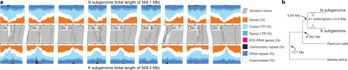
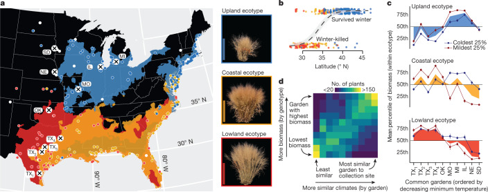
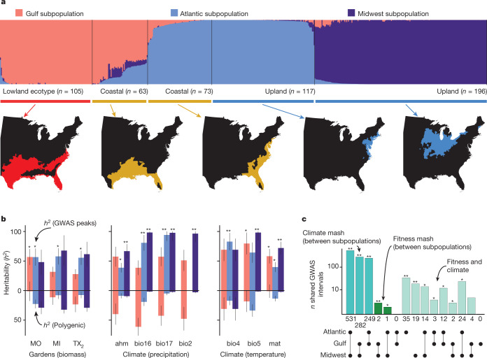
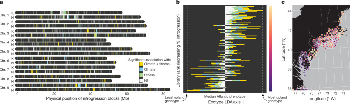
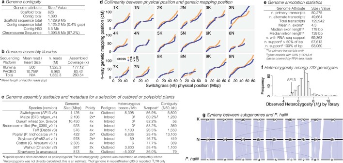
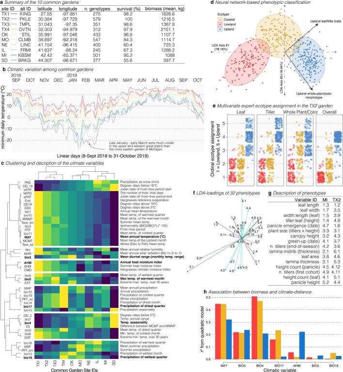
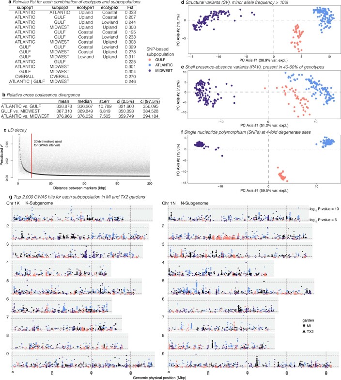
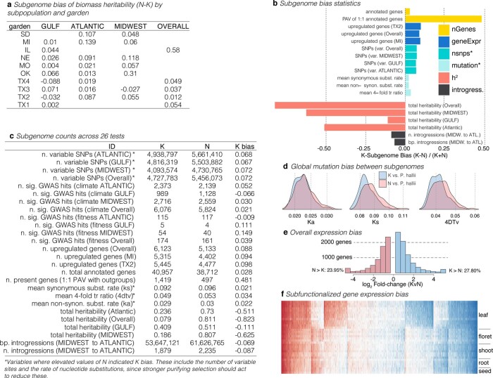
Long-term climate change and periodic environmental extremes threaten food and fuel security¹ and global crop productivity^2-4. Although molecular and adaptive breeding strategies can buffer the effects of climatic stress and improve crop resilience⁵, these approaches require sufficient knowledge of the genes that underlie productivity and adaptation⁶-knowledge that has been limited to a small number of well-studied model systems. Here we present the assembly and annotation of the large and complex genome of the polyploid bioenergy crop switchgrass (Panicum virgatum). Analysis of biomass and survival among 732 resequenced genotypes, which were grown across 10 common gardens that span 1,800 km of latitude, jointly revealed extensive genomic evidence of climate adaptation. Climate-gene-biomass associations were abundant but varied considerably among deeply diverged gene pools. Furthermore, we found that gene flow accelerated climate adaptation during the postglacial colonization of northern habitats through introgression of alleles from a pre-adapted northern gene pool. The polyploid nature of switchgrass also enhanced adaptive potential through the fractionation of gene function, as there was an increased level of heritable genetic diversity on the nondominant subgenome. In addition to investigating patterns of climate adaptation, the genome resources and gene-trait associations developed here provide breeders with the necessary tools to increase switchgrass yield for the sustainable production of bioenergy.

Fig. 1. The structure and evolution of the subgenomes of tetraploid switchgrass.

a, Grey polygons (representing n = 53 syntenic blocks) demonstrate nearly complete co-linearity between subgenomes. Gene-rich chromosome arms and highly repetitive pericentromeres are typical of grass genomes. LTR, long-terminal repeat. b, Subgenome divergence of <4.6 Ma was estimated from a time-scaled phylogenetic tree calibrated to the Panicum–Setaria node at 13.1 Ma. Source data

Fig. 2. Climatic adaptation within and among switchgrass ecotypes.

a, Geographical distribution of common gardens (n = 10) and plant collection locations (n = 700 georeferenced genotypes), and spatial distribution models of each ecotype. The ecotype colour legend accompanies the representative images of each ecotype to the right of the map (images were taken at the end of the 2019 growing season and the background was removed with ImageJ (https://imagej.nih.gov/ij)). White-outlined points (coloured by ecotype, or in white if no ecotype assignment was made) indicate the georeferenced collection sites of the diversity panel. The labelled white circles with black crosses indicate the locations of the 10 experimental gardens. Publicly available cultural and physical geographical information system (GIS) layers were accessed with the rnaturalearthdata R package. Scale bars, 1 m. b, Across the landscape, survival (n_genotypes = 367) and winter kill (n = 184) in the northern gardens (n = 3) was geographically structured: the latitude of the origin of collection site was predictive of survival. A logistic regression prediction (±s.e.) accompanies binary survival along the latitude predictor. c, Imputed survival-corrected biomass was converted to percentiles for each ecotype (0 = lowest biomass, 100 = highest) and mean percentiles were plotted overall (coloured polygons, n = 447) for each ecotype (n_upland = 211, n_coastal = 144, n_lowland = 92) and garden. The biomass percentiles (mean ± s.e.m.) for the 25% of genotypes from sites with the coldest extreme 30-year coldest minimum temperature (blue lines and points) (n_upland = 52, n_coastal = 35, n_lowland = 22) and the mildest 25% (red lines and points) (n_upland = 53, n_coastal = 36, n_lowland = 23) demonstrate that climate of origin affects biomass within ecotypes and across gardens. d, A heat map of the rank of climate similarity (x axis) and imputed biomass (y axis) demonstrates that the majority of 571 genotypes achieve their highest biomass at common gardens that were climatically similar to their source habitat. Source data

Fig. 3. Population and quantitative genomics of climate-associated adaptation.

a, Admixture proportions among three gene pools (coloured by subpopulation) and three ecotypes (labelled below), calculated using eigenvector decomposition of the identity-by-descent matrix. The corresponding geographical distribution of each ecotype is presented below the bar plot (coloured by the ecotype distributions from Fig. 1a). Publicly available cultural and physical GIS layers were accessed with the rnaturalearthdata R package. b, Post hoc tests of SNP–heritability (mean h² ± s.e.m.) attributable to polygenic background (below the black horizontal lines) and significant multivariate adaptive shrinkage GWAS hits (above the black horizontal lines) are presented for the three main sites (biomass) and for precipitation- and temperature-related climate variables, and coloured by subpopulations (following a). Extended Data Fig. 2c provides descriptions of the climate variables (ahm, bio2, bio4, bio5, bio16, bio17 and mat). Statistical significance of higher heritability for GWAS hits relative to polygenic inheritance is indicated for two-sided Z-score P values; **P < 0.001, *P < 0.05. c, There are large and significant overlaps in climate-associated multivariate adaptive shrinkage (mash) intervals between subpopulations, and smaller but significant overlaps between fitness and climate hits in the Atlantic and Midwest subpopulations. Two-sided Fisher’s test P value significance, following b. Source data

Fig. 4. Mapping the location and effect of Midwest introgressions in the Atlantic subpopulation.

a, Positions of all high-frequency (present in >10 genotypes, n = 1,640) introgressions from Midwest into the Atlantic subpopulation are coloured by significance in the two redundancy analyses for climate (blue, n = 234), biomass and survival (green, n = 329) or ‘climate–fitness overlap’, which are significant in both (gold, n = 245). NS, not significant. b, Introgressions are strongly associated with a more upland phenotype among 135 genotypes. For each genotype, the position along the first discriminant axis between ecotypes (Extended Data Fig. 2) is scaled relative to the median Atlantic ecotype value, then plotted and coloured by the proportion of introgressed sequence in each significance bin from a. c, The introgression ranks from b were converted to a purple–orange colour scale (right of b) and georeferenced positions of collection sites for each library are plotted for the northern Atlantic seaboard of the USA. Publicly available cultural and physical GIS layers were accessed with the rnaturalearthdata R package. Source data

Extended Data Fig. 1. Genome assembly and annotation.

a–c, Genome contiguity (a) and library coverage (b) demonstrate that the v5 release is a very complete genome and that it is among the best available plant reference genomes (c), compared to maize durum wheat, broomcorn millet, teff, poplar, soybean, cotton, walnut and strawberry. d, Complete collinearity between marker order in both crosses (number of markers = 4,701) of a 4-way mapping population is evident. e, Genome annotation statistics present a gene annotation that is as complete as the assembly. f, Observed heterozygosity ranges from <4 to >10% among our 732-library resequencing panel. g, Nearly the entire single-copy genome of P. hallii is syntenic with both switchgrass subgenomes; pale blue polygons represent syntenic blocks between subgenomes and P. hallii. The one exception is a previously known over-retained region representing the ρ duplication on Chr. 03 and 08. Source data

Extended Data Fig. 2. Phenotypic and climatic gradients among common gardens and ecotypes.

a, The ten common gardens span much of the geographical distribution of, and elicit very different phenotypic responses among, our switchgrass diversity panel. For each garden, we present the georeferenced location and some basic quantitative genetic attributes of the plants grown there. b, To illustrate the climate context of winter mortality, we present a seven-day rolling mean of minimum daily temperature across the study period. Line colours match the colour key in a. c, To investigate the climatic attributes of each garden, we clustered 46 climatic variables from WorldClim (variables are named bio1–19) and ClimateNA using the georeferenced locations for the diversity panel; the identifiers (left) and description (right) accompany each row. These seven clusters, separated by breaks in the heat map, are represented by the seven climate variables that most closely correlated with the first principal component eigenvector of each cluster (labelled in bold). d, To investigate ecotype evolution, we probabilistically assigned each member of the diversity panel to one of three ecotypes (n_upland = 221, n_coastal = 157, n_lowland = 129) using a set of morphological (n = 16 at 2 gardens) and qualitative (n = 2) phenotypes; the linear discriminant functions that distinguish the ecotypes are presented here along with the eigenvectors of the two qualitative ecotype categorizations. Each point represents a single genotype grown in both TX₂ and MI gardens (n = 509). LDA, linear discriminant analysis. e, Qualitative ecotype assessments from experts are presented for the TX₂ garden in 2019. The y-axis scale is ordinal with five categories, but points are jittered so that the density of observations is more obvious. Points are coloured by neural network classification following d. f, Loadings for the other 16 variables (across 2 gardens) are plotted on the same scale and axes as d. To distinguish variables, we clustered each into one of four groups, representing variation in leaf (dark green) (3), whole plant (red) (1) and combinations of these. g, The table presents a legend for the labels in f, in which each variable was measured in both MI and TX₂ gardens. More detailed descriptions of the phenotypes can be found in Supplementary Data 5. h, For each of the seven climate variables, we corrected climate distance between the collection site and each common garden. The quadratic model fit (r²) for each variable and ecotype are presented. Source data

Extended Data Fig. 3. Population and quantitative genetic divergence between and evolution within subpopulations and ecotypes.

a, Pairwise F-statistics between each subpopulation-by-ecotype combination and across all ecotypes for each subpopulation. b, Cross coalescence (RCCR) represents an alternative method to define divergence. Here, 16 bootstraps of RCCR profiles were converted to generation time at which divergence occurred. Statistics across the bootstraps are presented. c, Linkage-disequilibrium nonlinear function of physical distance and predicted correlation coefficients among markers for the entire sample. The linear model prediction for each 500-bp interval is plotted as black open points; 2-bp-interval mean r² values are the light grey points in the background. d–f, Population genetic structure is displayed as the principal coordinates from a scaled and centred distance matrix of structural variants (d), presence–absence variants (e) and SNPs (f), colour-coded by subpopulation assignments in Fig. 3. g, Positions and −log₁₀(P values) of the top 2,000 GWAS hits are presented for 2 gardens, the 3 subpopulations (coloured as in d–f) and an overall run (black points). Source data

Extended Data Fig. 4. Subgenome biases across DNA, expression and quantitative traits.

a, Difference in biomass SNP–heritability (h²) estimates between subgenomes for each garden-by-subpopulation combination. Garden-by-subpopulation combinations with empty cells indicate that the model did not converge. b, Subgenome bias for all sets of genome analyses conducted here. Colours indicate the dataset used. c, Counts and ratios used to build b, with longer descriptions of the variables. d, Density distributions of nonsynonymous (K_a), synonymous (K_s) and fourfold-degenerate transversion substation rates (4DTv) for each subgenome relative to P. hallii. e, Summation of the number of genes in each colour bin of f. f, A heat map of expression in which K > N (blue) and N > K (red) is shown for each tissue in the genome-annotation RNA-seq dataset. Source data

References

1. Lobell DB, Schlenker W, Costa-Roberts J. Climate trends and global crop production since 1980. Science. 2011;333:616–620. doi: 10.1126/science.1204531. - DOI - PubMed
1. Challinor AJ, et al. A meta-analysis of crop yield under climate change and adaptation. Nat. Clim. Chang. 2014;4:287–291. doi: 10.1038/nclimate2153. - DOI
1. Rosenzweig C, et al. Assessing agricultural risks of climate change in the 21st century in a global gridded crop model intercomparison. Proc. Natl Acad. Sci. USA. 2014;111:3268–3273. doi: 10.1073/pnas.1222463110. - DOI - PMC - PubMed
1. Porter, J. R. et al. in Climate Change 2014: Impacts, Adaptation, and Vulnerability. Part A: Global and Sectoral Aspects (Contribution of Working Group II to the Fifth Assessment Report of the Intergovernmental Panel on Climate Change) (eds Field, C. B. et al.) 485–533 (Cambridge Univ. Press, 2014).
1. Bevan MW, et al. Genomic innovation for crop improvement. Nature. 2017;543:346–354. doi: 10.1038/nature22011. - DOI - PubMed
Publication types