A data reduction and compression description for high throughput time-resolved electron microscopy

Abstract

Fast, direct electron detectors have significantly improved the spatio-temporal resolution of electron microscopy movies. Preserving both spatial and temporal resolution in extended observations, however, requires storing prohibitively large amounts of data. Here, we describe an efficient and flexible data reduction and compression scheme (ReCoDe) that retains both spatial and temporal resolution by preserving individual electron events. Running ReCoDe on a workstation we demonstrate on-the-fly reduction and compression of raw data streaming off a detector at 3 GB/s, for hours of uninterrupted data collection. The output was 100-fold smaller than the raw data and saved directly onto network-attached storage drives over a 10 GbE connection. We discuss calibration techniques that support electron detection and counting (e.g., estimate electron backscattering rates, false positive rates, and data compressibility), and novel data analysis methods enabled by ReCoDe (e.g., recalibration of data post acquisition, and accurate estimation of coincidence loss).

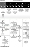
Fig. 1. Data reduction levels and scheme.

a The leftmost image (L0) depicts a 10 × 10 pixel image (the raw detector output) with four secondary electron puddles. The remaining four images from left to right correspond to the four data reduction levels, L1 to L4, respectively. Each image represents a reconstruction of the original image (L0) using only the information retained at that level (see table at the bottom). The L1 image retains all the useful information about the secondary puddles by first removing detector readout/thermal noise from L0. In L2, the spatial location of the four puddles, the number of pixels (area) in each puddle, the shape of the four puddles and an intensity summary statistic (sum, maximum or mean) for each puddle are retained. Each reduction level offers different advantages in terms of speed, compression, information loss, spatial or temporal resolution, etc (see row labeled “Optimized For”). The row labeled “Reduced Representation” describes how the information retained at each level is packed in the reduced format. These packings are tuned to provide a good balance between reduction speed and compressibility. In L3, the puddle area, shape and location information are all encoded in a single binary image, which is easily computed and highly compressible. These three aspects in L1 and L2 are packed as the binary image used in L3. Only the most likely locations of incident electrons are saved as binary maps in L4. Panels b, c, d, and e are the reduction compression pipelines for reduction levels L1, L2, L3, and L4, respectively. Here, the thresholding step produces a binary map identifying pixels as signal or noise. Bit packing removes unused bits and converts the list of ADU values into a continuous string of bits. The connected components labeling algorithm identifies clusters of connected pixels that constitute individual electron puddles from this binary map. Puddle centroid extraction further reduces each puddle to a single representative pixel; and puddle feature extraction computes puddle specific features such as mean or maximum ADU.

Fig. 2. Recalibration of L1 reduced data to remove artifacts.

Panels a and b are Fourier transforms (FT) of summed L1 reduced frames of HRTEM movies of a molybdenum disulfide 2-D crystal, acquired using a JEOL 2200 microscope operating at 200 keV and a DE-16 detector running at 300 fps, with a pixel resolution of 0.2□ (a) is L1 reduced using fast on-the-fly calibration using a 3□ threshold (see “Methods” section) (b) is the result of recalibrating (a) with a more stringent fine calibration that uses an area threshold and a 4□ threshold (see “Methods” section). The Fourier peaks indicated with orange arrows in a are due to detector artifacts, which are not readily visible in the image but can severely impact drift correction. a and b are the sum of FFTs of 9000 frames.

Fig. 3. Reducibility and compressibility of data with increasing electron flux.

The solid black line (“unreduced compression”) shows the compression ratios achieved on unreduced raw data (including dark noise) using Deflate-1. The dashed lines show the compression ratios achieved with just the four levels of data reduction and without any compression. The solid lines show the compression ratios after compressing the reduced data using Deflate-1. The coincidence loss levels corresponding to the electron fluxes label the second y-axis on the right.

Fig. 4. Comparison of compression algorithms with L1 reduction at three dose rates.

Each scatter plot shows the reduction compression ratios and the compression throughputs of six compression algorithms (Deflate, Zstandard (Zstd), bzip2 (Bzip), LZ4, LZMA, and SNAPPY), plus the Blosc variants of Deflate, Zstandard (Zstd), LZ4, and SNAPPY. Reduction compression ratio (horizontal axes in all panels) is the ratio between the raw (uncompressed) data and the reduced compressed data sizes. The three rows of scatter plots correspond to three different electron fluxes: 0.01, 0.03, and 0.05 e/pixel/frame, from top to bottom. The left and right columns of scatter plots correspond to the two most extreme internal optimization levels of the compression algorithms: fastest but suboptimal compression labeled “Optimal Speed” (left column), and optimal but slow compression labeled “Optimal Compression” (right column). The data throughputs (vertical axes in all panels) are based on single threaded operation of ReCoDe and include the time taken for both reduction and compression. The decompression throughputs of the six algorithms are presented in Supplementary Fig. 2.

Fig. 5. Pipeline and data throughput of on-the-fly reduction and compression.

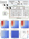
a ReCoDe’s multithreaded reduction compression pipeline used for live data acquisition. The CMOS detector writes data into the RAM-disk in timed chunks, which the ReCoDe server processes onto local buffers and then moves to NAS servers. The ReCoDe Queue Manager synchronizes interactions between the ReCoDe server and the detector. b L1 reduction and compression throughput (GB/s) of Deflate-1, with multiple cores at four electron fluxes. The throughput of ReCoDe depends only on the number of electron events every second, hence the four dose rates (horizontal axis) are labeled in million electrons/second. The simulations were performed on a 28-core system, as a result, throughput scales non-linearly when using more than 28 cores (Supplementary Fig. 3). c, d Show throughputs when using 10 GbE and IPoIB connections to write directly to NAS, respectively. In e, throughput of L1 reduction without any compression; (f) throughput of Deflate-1 when compressing the unreduced raw data. g Shows the conversion between million e/s and e/pixel/frame for two different frame size-frame rate configurations of the DE-16 detector.

Fig. 6. Maximum data acquisition time of 1 TB of movie-mode TEM without data reduction and compression.

Each cell’s horizontal and vertical grid position marks the temporal resolution (or, equivalently, frame rate) and frame size of a hypothetical movie-mode data acquisition scenario, respectively. A cell’s text and color indicates the time taken to acquire one terabyte (TB) of data at that frame size and temporal resolution without reduction and compression. For larger frames and high temporal resolution (top right corner), acquisitions lasting merely tens of seconds already produce 1 TB of data. With a 95× reduction in data size the same experiment can span 20 times longer, enabling the observation of millisecond dynamics in reactions that span several minutes. The yellow dots show a few of the frame size-frame rate combinations available for the DE-16 detector.

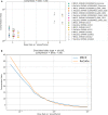
Fig. 7. Comparison of ReCoDe and MRCZ for archival datasets in EMPIAR.

a Shows that the compression ratios obtained by ReCoDe (filled stars) on relatively low dose rate EMPIAR datasets are higher than those due to MRCZ (filled circles). b Compression ratios obtained using MRCZ and ReCoDe on simulated 16-bit unsigned integer data. The crossover point for performance occurs at 0.58 electron/pix/frame. At dose rates below this ReCoDe achieves higher compression ratios than MRCZ, whereas at dose rates above this MRCZ achieves slightly higher compression ratios. The number of electron events per pixel follows a Poisson distribution in these simulated datasets. The underlying compression algorithms used in a and b is Blosc + Deflate (zlib) for both MRCZ and ReCoDe. Table 2 lists a short description of the seven EMPIAR dataset used to generate (a). Overall in the simulated data, for both compression algorithms, compression ratios reduce as dose rate increases, as expected. However, for the EMPIAR datasets, there are two groups, one for the floating-point data (datasets 0–5) and another for integer data (datasets 6 and 7). Although the floating-point data have lower dose rates than the integer type data, the former is less compressible because they are naturally less sparse than the latter. Nevertheless, within each group, the expected trend (reduction in compression ratio with increasing dose rate) holds true and ReCoDe outperforms MRCZ. A comparison where all the datasets are standardized to the same integer data type, presented in Supplementary Fig. 6, shows that the results from EMPIAR datasets and simulated data are quite similar.

References

1. Datta A, Chee SW, Bammes B, Jin L, Loh D. What can we learn from the shapes of secondary electron puddles on direct electron detectors? Microsc. Microanal. 2017;23:190–191. doi: 10.1017/S1431927617001635. - DOI
1. Li X, Zheng SQ, Egami K, Agard DA, Cheng Y. Influence of electron dose rate on electron counting images recorded with the K2 camera. J. Struct. Biol. 2013;184:251–260. doi: 10.1016/j.jsb.2013.08.005. - DOI - PMC - PubMed
1. Johnson, I. J. et al. Development of a fast framing detector for electron microscopy. In 2016 IEEE Nuclear Science Symposium, Medical Imaging Conference and Room-Temperature Semiconductor Detector Workshop (NSS/MIC/RTSD) 1–2 (IEEE 2016).
1. Chee SW, Anand U, Bisht G, Tan SF, Mirsaidov U. Direct observations of the rotation and translation of anisotropic nanoparticles adsorbed at a liquid-solid interface. Nano Lett. 2019;19:2871–2878. doi: 10.1021/acs.nanolett.8b04962. - DOI - PubMed
1. Levin BDA, Lawrence EL, Crozier PA. Tracking the picoscale spatial motion of atomic columns during dynamic structural change. Ultramicroscopy. 2020;213:112978. doi: 10.1016/j.ultramic.2020.112978. - DOI - PubMed
LinkOut - more resources