Regulatory genomic circuitry of human disease loci by integrative epigenomics

Abstract

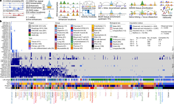
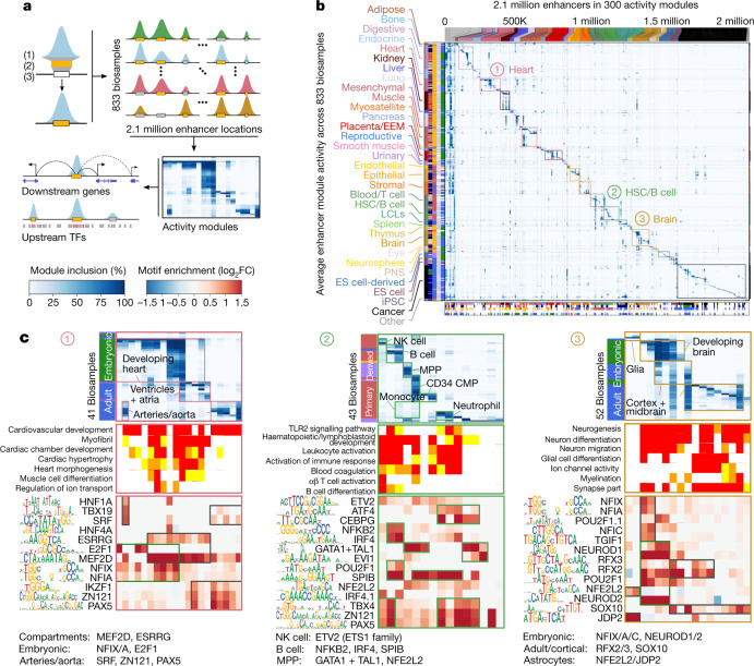
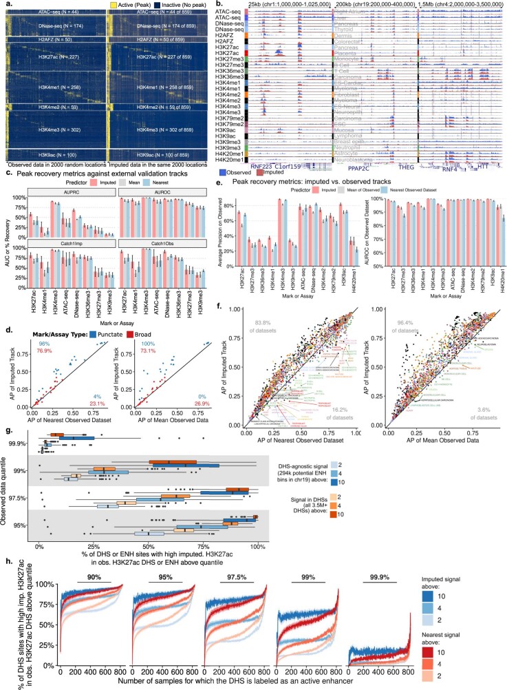
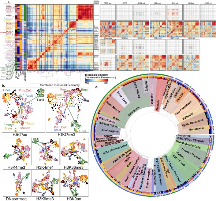
Annotating the molecular basis of human disease remains an unsolved challenge, as 93% of disease loci are non-coding and gene-regulatory annotations are highly incomplete^1-3. Here we present EpiMap, a compendium comprising 10,000 epigenomic maps across 800 samples, which we used to define chromatin states, high-resolution enhancers, enhancer modules, upstream regulators and downstream target genes. We used this resource to annotate 30,000 genetic loci that were associated with 540 traits⁴, predicting trait-relevant tissues, putative causal nucleotide variants in enriched tissue enhancers and candidate tissue-specific target genes for each. We partitioned multifactorial traits into tissue-specific contributing factors with distinct functional enrichments and disease comorbidity patterns, and revealed both single-factor monotropic and multifactor pleiotropic loci. Top-scoring loci frequently had multiple predicted driver variants, converging through multiple enhancers with a common target gene, multiple genes in common tissues, or multiple genes and multiple tissues, indicating extensive pleiotropy. Our results demonstrate the importance of dense, rich, high-resolution epigenomic annotations for the investigation of complex traits.

Fig. 1. EpiMap resource overview.

a, We created a compendium of over 17,000 epigenomic tracks across 18 marks by uniform processing and imputation and used these to call chromatin states for 833 biosamples and active-enhancer states over 2.1 million DNase I hypersensitive sites (DHSs). We used unsupervised clusters of the enhancer activities to call enhancer downstream target genes, upstream regulators, and to prioritize, investigate and compare hundreds of GWAS traits and thousands of loci. GO, gene ontology; QC, quality control; TF, transcription factor. b, Data matrix across 859 samples (columns) and 40 assays (rows), ordered by the number of experiments (parentheses) and coloured by metadata. EEM, extra-embryonic membranes; ES, embryonic stem; expts, experiments; HSC, haematopoietic stem cell; iPSC, induced pluripotent stem cell; H3T11ph, histone H3 phosphorylated at T11; PNS, peripheral nervous system. ENCODE new, ENCODE post-2012 data freeze + publication; Roadmap new, Roadmap post-2015 data freeze + publication.

Fig. 2. Enhancer module circuitry.

a, Overview of gene-regulatory module clustering. The full module breakdown is shown in Extended Data Figs. 6, 7 and online at http://compbio.mit.edu/epimap. Activity modules are shown in Fig. 2b, Extended Data Fig. 6a. FC, fold change. b, Clustering of 2.1 million enhancer elements (top) into 300 modules (columns) using the activity levels of enhancers (heat map) across 833 samples (rows), quantified by the levels of H3K27ac within accessible enhancer chromatin states. Bottom, the enrichment of each module for each metadata annotation, highlighting 34 groups of modules (separated by dotted lines): 33 specific to sample type (coloured boxes) and 1 multiply enriched (left-most). LCL, lymphoblastoid cell line. c, Subsets of enhancer module centres (top panels) and motifs (bottom panels) for heart, brain and haematopoietic cell samples (top, rows), selected GO terms (middle, rows) and selected motifs (bottom, rows) in modules (columns) with maximal enrichment in each of the three sample categories. The GO heat map is coloured by enrichment −log₁₀P (0–2: white; 2–3: yellow; 3–4: orange; and 4+: red). The full subsets are shown in Extended Data Fig. 7. CMP, common myeloid progenitor; MPP, multipotent progenitor; NK, natural killer.

Fig. 3. Trait–trait network.

The network across 215 traits (FDR < 1%) by similarity of epigenetic enrichments (cosine similarity ≥ 0.75), laid out using the Fruchterman–Reingold algorithm. Only 215 connected traits are shown. Traits (nodes) are coloured by the contributing groups (pie chart by the fraction of −log₁₀P, and size by maximal −log₁₀P) and interactions (edges) by the group with the maximal dot product of enrichments between two traits. The redundant node names indicate different GWAS (the full names for non-singleton nodes are available in Supplementary Fig. 22). AD, Alzheimer disease; ADHD, attention-deficit/hyperactivity disorder; BMI, body mass index; CVD, cardiovascular disease; FEV1, forced expiratory volume in 1 s; T2D, type 2 diabetes; vWF, von Willebrand factor; WHR, waist-to-hip ratio.

Fig. 4. Partitioning of polyfactorial traits.

a, Workflow for the investigation of GWAS epigenomic enrichment using the biosample tree (Extended Data Fig. 2c). Additional trait enrichments, SNP assignments, links and their corresponding loci are available at http://compbio.mit.edu/epimap. b, Epigenomic enrichments for CAD on the enhancer-sharing tree. Nodes that passed false discovery rate <1% are labelled by rank, category and components, and subtrees are shown (the large circles are the top 20 nodes by −log₁₀P). The leaves are annotated by metadata and the number of enriched parent nodes (outer circle is red to black with increasing number of parent nodes; inner circle is green if the leaf has an epigenome-level enrichment). c, The top 10 enriched nodes for CAD with nominal P values (heat map) and shared enhancer set sizes (bar plot) with the number at the subtree (full bar) and the number of differential enhancers between the node and its parent (tested set, dark bar). d, GO enrichments of node enhancers with lead SNPs (nearest expressed genes), coloured by the tissue group of each node and diagonalized (over-representation test). e, Enrichment for significant loci in overlap of CAD loci with loci from five related traits, within enriched enhancers in each node (heat map, −log₁₀P of one-tailed Mann–Whitney test against the loci of each trait in the enhancer annotations). f, Enhancer overlaps with the top 30 lead SNPs from CAD GWAS for the top 10 enrichments on the enhancer tree. g–i, Loci centred on CAD lead SNPs with links (top), the H3K27ac signal (middle) and GWAS summary statistics, for lead SNPs rs2107595 (chr7:19,049,388, P = 1 × 10⁻²⁴) (g), rs6841581 (chr4: 148,401,190; P = 5 × 10⁻²⁴) (h) and rs3184504 (chr12:111,884,608, P = 5 × 10⁻³⁰) (i). Loci show enhancer–gene links for SNP proximal enhancers for the top enrichments (Enr.) and across the locus for labelled categories (Cat.; linked enhancers in grey) (top); the H3K27ac signal in enhancers for the top three enriched subtrees, the six selected tissue categories and the average (middle); and genes (transcription start site (red lines)) and CAD GWAS summary statistics, with SNPs below P = 5 × 10⁻⁸ in grey (bottom).

Extended Data Fig. 1. Imputation validation.

a, Heat map of paired observed and imputed signal intensity across all punctate Tier 1 and Tier 2 assays across 2000 highest-max-signal bins among 5000 randomly-selected 25bp bins. Samples (rows) and bins (columns) are clustered and diagonalized using maximum imputed signal intensity, with broadly-active regions shown first. b, Paired observed (blue) and imputed (red) tracks for all Tier 1 and Tier 2 assays in three regions at different resolutions for randomly-selected samples. Each row shows a single track across three different resolutions. Full tracks at https://epigenome.wustl.edu/epimap. c, Genome-wide imputation performance metrics for predicting 51 external validation tracks across 8 assays in 14 biosamples (average precision, AUROC predicting top 1% of observed data and peak recovery of top 1% Imputed or Observed with top 5% Observed or Imputed, respectively) in chr1, shown for either the appropriate imputed track, the best-matching of the other observed tracks, or the observed signal average. d, Scatter comparison of average precision (AP) of imputed data with either nearest observed track or signal average in punctate (blue) and broad (red) marks. e, Genome-wide imputation performance metrics (AP, AUROC) for predicting observed tracks (evaluated on all observed tracks with an imputed prediction) in chr19, shown for either the appropriate imputed track, the best-matching of the other observed tracks, or the observed signal average. f, Scatter comparison of average precision (AP) of imputed data with either nearest observed track or signal average across all datasets, coloured by sample group. Cases where the nearest sample or the mean heavily outperformed the imputation are labelled (points with over 25%, for nearest, or 10%, for mean, greater average precision than the imputed track). g, Sample-specific percentage of the 2M DHSs with imputed H3K27ac above a certain cut-off that are also in the top 10%, 5%, 2.5%, 1%, and 0.1% of 3.6M DHSs by matched observed datasets. h, Sample-specific percentage of the 2M DHSs with imputed (blue) or nearest observed (red) H3K27ac above a certain cut-off that are also in the top 10%, 5%, 2.5%, 1%, and 0.1% of 3.6M DHSs by matched observed datasets, partitioning the DHSs by the number of samples in which each DHS is called as an active enhancer.

Extended Data Fig. 2. Cross-sample relationships.

a, Hierarchically clustered genome-wide correlation across samples in all 13 imputed Tier 1 and 2 assays. Observed (top) vs. imputed (bottom) matrices shown. Clustering conducted on the fused matrix (left panel, constructed as in main figure). Observed data availability matrix (grey is available, white is unavailable) is shown for the top nine marks and accessibility assays by number of observed datasets. b, Two-dimensional embeddings of Tier 1 and 2 marks coloured by tissue group, using Spearman correlation within matched chromatin states. Arrows point from the centre of mass of all biosamples to that of the specified group. c, Hierarchical clustering of 833 biosamples based on enhancer activity distances (Supplementary Fig. 12). Subtrees enriched for specific sample types are highlighted and labelled (colours). Samples are labelled by metadata in the outer ring (Supplementary Table 1).

Extended Data Fig. 3. Chromatin states.

a, Epigenomic state mnemonics for ChromHMM 18-state model (left) with emissions matrix (centre) and state definitions (right). The 18-state model was trained on Roadmap data for the Roadmap 2015 paper. b, Distributions of per-state genome coverage (box-plots) across 833 biosamples (points, coloured by tissue group) according to the ChromHMM 18-state model annotations. c, Genome coverage for each 18-state-model ChromHMM state across 833 biosamples after QC. Lower panel shows availability of 9 top marks, ordered by the number of observed datasets. Biosamples are ordered by per cent of the genome not annotated as quiescent. d, Comparison of per state (left panel) model emissions (middle panel) against mark occurrence in state calls (right panel) across 833 biosamples (columns in right panel). Observed occurrence matched the emissions closely, with three exceptions, corresponding to bivalent chromatin states and transcribed enhancers (cumulatively covering 0.48% of the genome on average), which showed discrepancies for 12.1% of biosamples on average, likely stemming from their low frequency in the genome, and the frequent co-occurrence of H3K27ac and H3K4me1.

Extended Data Fig. 4. Comparison with SCREEN.

a, Recovery of each category of SCREEN elements by each category of EpiMap elements, percentage (left) and number (right). b, Recovery of each category of EpiMap elements by each category of SCREEN elements, percentage (left) and number (right). c, Percentage of EpiMap enhancers in dELS in each of 300 modules and 833 epigenomes. d, Percentage of EpiMap enhancers in dELS by number of epigenomes containing element (blue line represents loess smooth). e, Comparison of motif-module log2 fold change enrichments for all enhancers and for the intersection of enhancers and dELS. f–i, Comparison of enhancer sets within EpiMap enhancers (intersections with dELS, non-dELS, unique, and all enhancers), showing percentage of 113k pruned GWAS catalogue lead SNPs within 2.5kb of enhancer centres (f), per cent of enhancers with a GWAS SNP within 2.5kb of their centre (g), the distribution of distances of GWAS SNPs to their nearest enhancer within each set (h), and the number of SNPs for which the nearest enhancer fell into each of the constituent sets (i).

Extended Data Fig. 5. Enhancer-sharing sample tree.

Tree constructed from complete-linkage hierarchical clustering of Jaccard similarity matrix of enhancer activity across biosamples. Fifty subtrees covering the full tree are annotated with their major subgroups. Tree is cut and coloured to create 20 clusters for purposes of visualization. Leaves are labelled with metadata and reduced sample names and coloured according to their tissue group. Metadata (heat map track) from inside-out: tissue group, project, sample type, and donor sex and life stage.

Extended Data Fig. 6. Expanded enhancer module circuitry.

a, Clustering of 2.1M enhancer elements (top) into 300 modules (columns) using enhancer activity levels (heat map) across 833 samples (rows), quantified by H3K27ac levels within accessible enhancer chromatin states. Bottom panel shows enrichment of each module for each metadata annotation, highlighting 34 groups of modules (separated by dotted lines): 33 sample-type-specific (coloured boxes) and 1 multiply-enriched (left-most). b, Gene ontology^, (GO) enrichments (heat map) for each module (columns) across 865 terms (rows) with P < e-4. GO terms coloured by maximal enrichment group. Only 36 representative terms are shown, chosen by a bag-of-words approach within each tissue group. c, Motif enrichment (heat map) for each module (columns) across 160 motif clusters (rows) with enrichment log₂FC >1. Motifs coloured by module of maximal enrichment.

Extended Data Fig. 7. Expanded module enrichments and motif networks.

a–c, Enhancer module circuitry for heart (a), brain (b), and haematopoietic cells (c) expanding module subsets (Fig. 2d). From top to bottom, we show module centres for all samples in each group against all modules whose maximal inclusion lies in the group, motifs with over twofold enrichment (text: log₂FC), and GO enrichments for each module with tissue-category-specific enrichments. d, e, Snapshots of the motif-module network highlighting TEAD3 and HNF1A. Edges represent enrichments with log₂FC > = 1.5.

Extended Data Fig. 8. Linking statistics and validation.

a–f, Enhancer-gene linking statistics. a, Bar chart of median number of genes per enhancer per bin across biosamples. b, Bar chart of median number of enhancers per gene per bin across biosamples. c, Total number of sample groups in which a unique link is active, out of 3.3M unique links. d, Per cent of unique elements (enhancers or links) for which the element is active in a given number of biosamples. e, Median distance between the enhancer and TSS of a link per distance bin across biosamples. f, Mean or median link distance for all enhancers active in a given number of biosamples. All means represented by blue dashed lines and text and medians by red dashed lines and text. g, h, Comparison (prediction F1 score and AUPRC) of gene-enhancer link predictions (blue) with distance, activity by distance, correlation by distance, correlation and activity by distance, and Roadmap Epigenomic links on functional gene set-based links (g) and physical, genetic, and perturbation-based links across four cell lines (h).

Extended Data Fig. 9. GWAS tissue-prioritization.

a, Trait-tissue enrichment (centre, heat map) between reported lead single-nucleotide polymorphisms (SNPs) from 226 genome-wide association studies (rows) and accessible active enhancers across 833 biosamples (columns) (FDR <1%). Enriched tissue groups (left) and number of enriched biosamples (right) shown for each trait. Only 83 representative traits labelled, using a bag-of-words approach (full list of traits in Supplementary Fig. 19). Traits coloured by sample with maximal trait-tissue enrichment. b, Contribution of each project to the maximum GWAS trait-tissue enrichment for the 226 traits with significant enrichments. c, Enhancer overlaps with top 20 lead SNPs for breast cancer for top enrichments on the enhancer tree (FDR <5%). d, 1-Mb locus centred on breast cancer lead SNP rs17356907 (chr12:96027759, P = 1.0e-39) showing H3K27ac signal (middle panel) in enhancer DHSs for the top three enriched subtrees in the enhancer tree, six selected tissue categories, and overall average signal. TSSs indicated by red dashed lines. Top panel shows enhancer gene-links for SNP-proximal enhancers for the top enrichments and across the locus for epithelial, endothelial, and stromal cell biosamples. Linked enhancers are highlighted in grey. Bottom panel shows gene models and breast cancer GWAS summary statistics, with SNPs below P = 5e-8 in grey. e, Enhancer overlaps with top 20 lead SNPs for depressed affect for top enrichments on the enhancer tree (FDR <5%). f, 1-Mb locus centred on depressed affect lead SNP rs1261070 (chr18:52,903,085, P = 6.0 × 10⁻¹²), with links (top), H3K27ac signal (middle), and summary statistics as in d, with links for brain biosamples.

Extended Data Fig. 10. GWAS prioritization statistics.

a, Number of traits (y-axis) with significant GWAS trait-tissue enrichments for each combination (column) of projects (rows). b, Comparison of GWAS enrichments found (top) and number of significant trait-tissue pairs SNPs in significantly-enriched annotations (bottom) using different annotations within DHSs either without (left) or with H3K27ac signal (right). DNase-seq signal alone enriches for far fewer GWAS than enhancer states alone or with H3K27ac. c, Increase in the cumulative number of GWAS traits (y-axis) with significant trait-tissue enrichments with increasing numbers of biosamples (x-axis), ordered to maximize the number of novel trait annotations captured with each new biosample. Top 25 samples labelled and coloured by tissue group, with top 6 GWAS traits shown for the first 10 samples. Points coloured by project. All 226 traits are captured after inclusion of 50 samples. d, Increase in the cumulative number of GWAS traits (y-axis) with maximal trait-tissue enrichments with increasing numbers of biosamples (x-axis). All 226 traits are captured after inclusion of 115 samples. e, Comparison of GWAS enrichments found (y-axis, left) and number of lead SNPs in significantly-enriched annotations (y-axis, right) using different methodologies (x-axis) for two FDR cut-offs (shades).

Extended Data Fig. 11. Tissue-tissue GWAS relationships.

Principal and partner tissue enrichments. a, For each tree node label (rows), the number of GWAS traits (black x-axis, bottom) showing maximum enrichment in that tree node (dark bars, principal tissue) or any enrichment in that tree node (light bars, partner tissue), and the percentage of tissue-enriched traits for which the tissue shows the maximal enrichment (red x-axis, top) across 232 traits. b, Overlap in enriched GWAS traits between pairs of tissues with maximal enrichment in the trait (principal tissue, rows) and lower enrichment in the same trait (partner tissue, columns), using tree node labels. c, Top traits in significant interactions for selected tissue pairs (for liver, heart, adipose). For each pair of tissue groups we reported the top 5 GWAS by their per cent of significant enrichments coming from either group.

Extended Data Fig. 12. Extended CAD investigation.

a, Shared enrichments with CAD for 56 of 803 traits sharing at least two enrichments with the top 20 enriched nodes of CAD. Matrix is diagonalized according to maximal enrichment (nominal p-value, only enrichments passing FDR <1% are shown). b, Extended GO terms for CAD lead SNPs in enriched nodes. All GO terms with at least -log₁₀q >2 enriched in less than 25% of nodes.

References

1. Visscher, P. M. et al. 10 Years of GWAS discovery: biology, function, and translation. Am. J. Hum. Genet. 101, 5–22 (2017). - PMC - PubMed
1. Gallagher, M. D. & Chen-Plotkin, A. S. The post-GWAS era: from association to function. Am. J. Hum. Genet. 102, 717–730 (2018). - PMC - PubMed
1. Ward, L. D. & Kellis, M. Interpreting noncoding genetic variation in complex traits and human disease. Nat. Biotechnol. 30, 1095–1106 (2012). - PMC - PubMed
1. Buniello, A. et al. The NHGRI-EBI GWAS catalog of published genome-wide association studies, targeted arrays and summary statistics 2019. Nucleic Acids Res. 47, D1005–D1012 (2019). - PMC - PubMed
1. ENCODE Project Consortium. An integrated encyclopedia of DNA elements in the human genome. Nature489, 57–74 (2012). - PMC - PubMed
Publication types