CryoDRGN: reconstruction of heterogeneous cryo-EM structures using neural networks

Abstract

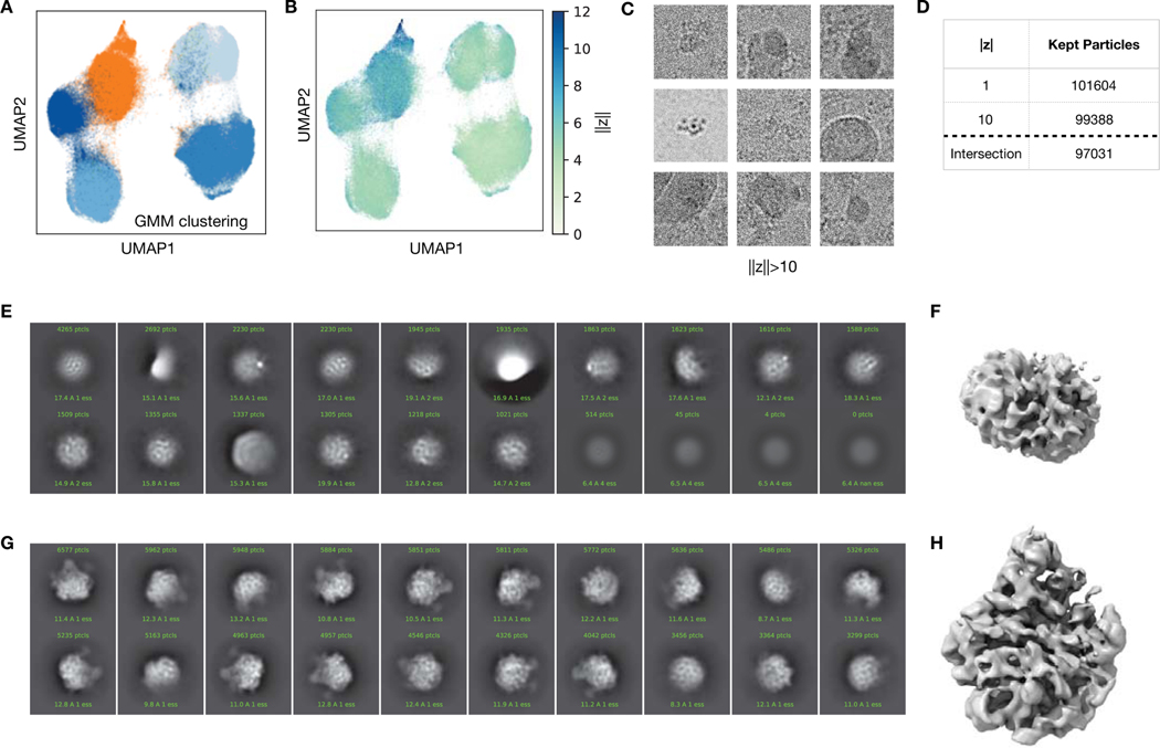
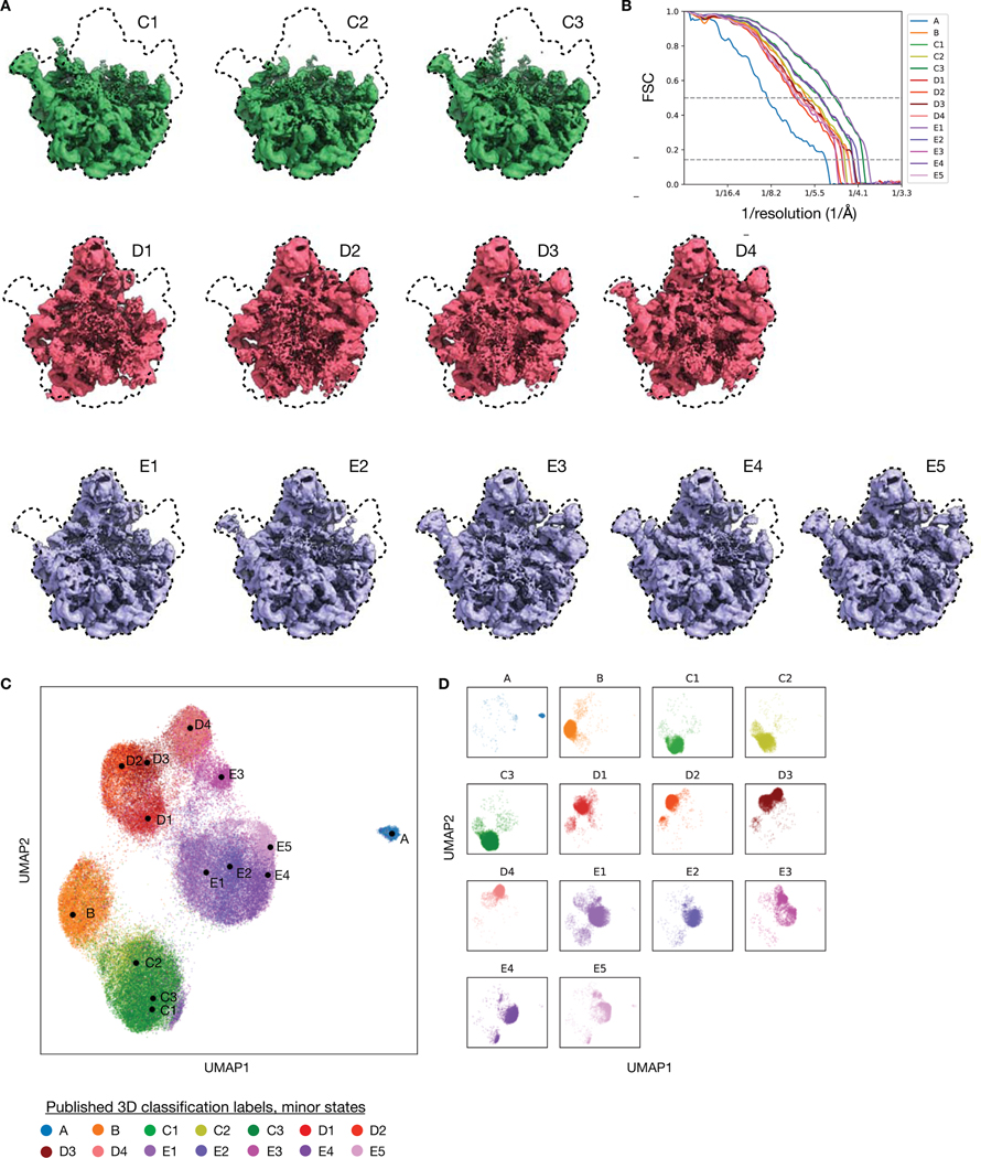
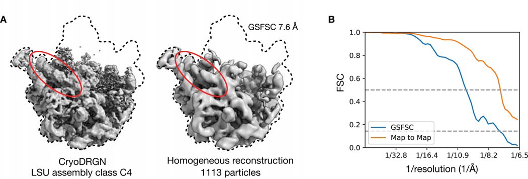
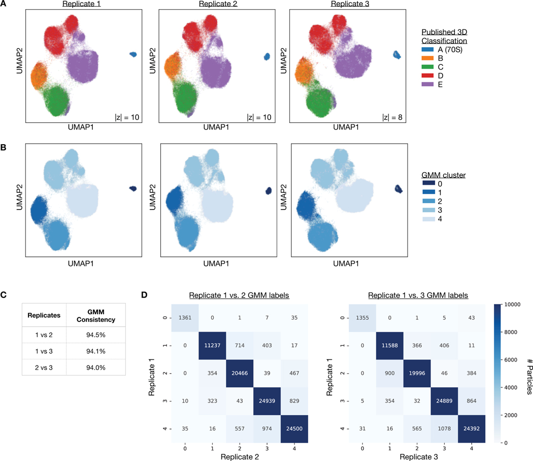
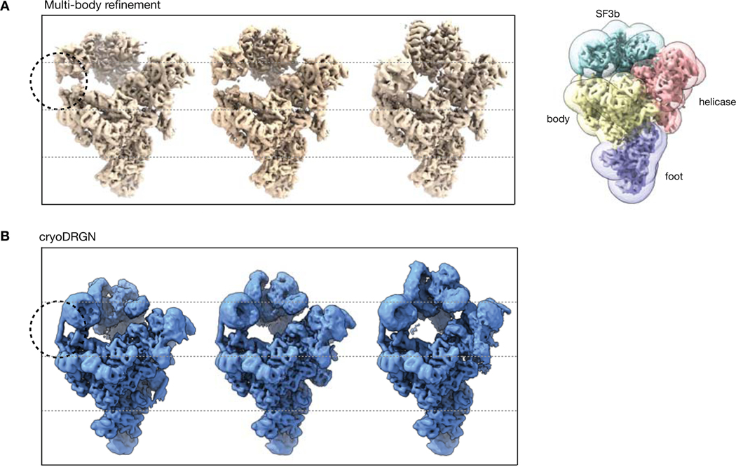
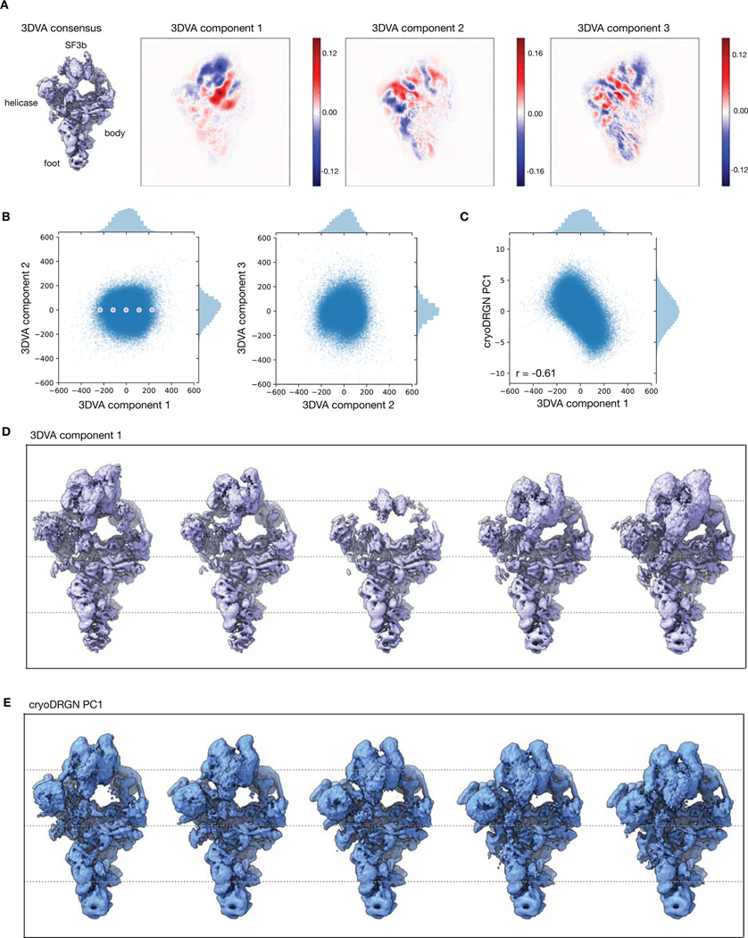
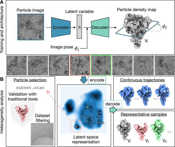
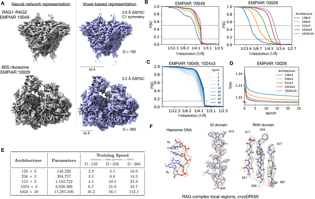
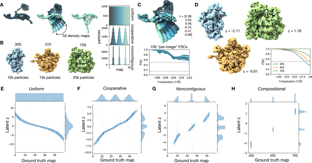
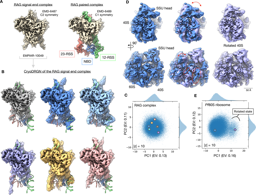
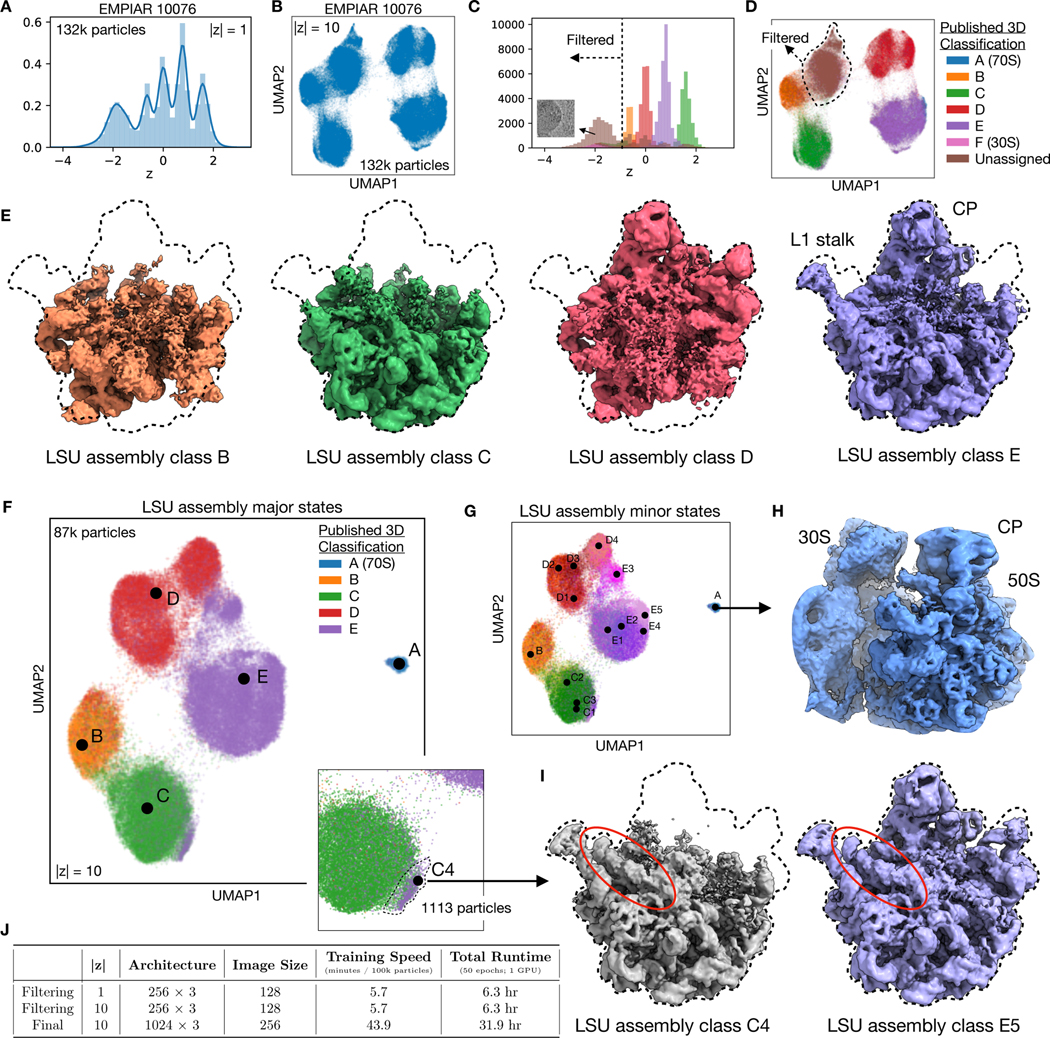
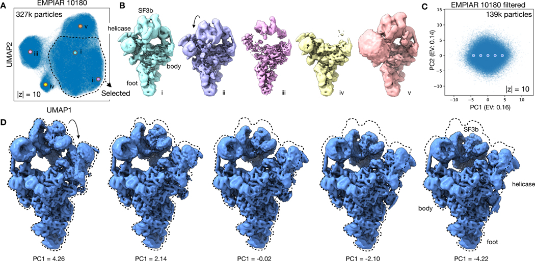
Cryo-electron microscopy (cryo-EM) single-particle analysis has proven powerful in determining the structures of rigid macromolecules. However, many imaged protein complexes exhibit conformational and compositional heterogeneity that poses a major challenge to existing three-dimensional reconstruction methods. Here, we present cryoDRGN, an algorithm that leverages the representation power of deep neural networks to directly reconstruct continuous distributions of 3D density maps and map per-particle heterogeneity of single-particle cryo-EM datasets. Using cryoDRGN, we uncovered residual heterogeneity in high-resolution datasets of the 80S ribosome and the RAG complex, revealed a new structural state of the assembling 50S ribosome, and visualized large-scale continuous motions of a spliceosome complex. CryoDRGN contains interactive tools to visualize a dataset's distribution of per-particle variability, generate density maps for exploratory analysis, extract particle subsets for use with other tools and generate trajectories to visualize molecular motions. CryoDRGN is open-source software freely available at http://cryodrgn.csail.mit.edu .

Extended Data Figure 1.. Per-image FSC curves between ground-truth maps and density maps from cryoDRGN trained on simulated heterogeneous datasets.

For each dataset, we compute 100 “per-image FSC curves” between generated and ground-truth density maps (Methods). Images are sampled at equally spaced percentiles along the reaction coordinate for the Uniform, Cooperative, and Noncontiguous datasets. For the Compositional dataset, the per-image FSC for 20, 30, and 50 randomly sampled images of the 30S, 50S, and 70S ribosome, respectively, are shown. No mask is used in computing the FSC.

Extended Data Figure 2.. RAG complex density maps reconstructed by cryoDRGN and by heterogeneous refinement in cryoSPARC.

A) Front (top) and back (bottom) view of the six cryoDRGN density maps of the RAG complex from Figure 4B. B) Density maps from 3D classification in cryoSPARC using the cryoDRGN density maps in (A) as initial models. Gold-standard FSC resolution and number of particles used in reconstruction are noted. C) Two side views of the density maps from 3D classification in (B), focusing on the RSS and NBD.

Extended Data Figure 3.. Missing head group of the Pf80S ribosome.

A) UMAP visualization of latent space encodings of EMPIAR-10028 particles with 50 sampled points shown in black. Sampled points are ordered according to distances in latent space (Methods). Visual inspection of the 50 volumes generated at the depicted points reveals 3 volumes with the 40S in a rotated state (purple) and 6 volumes with portions of the 40S head region missing (pink). B) Density map of the 80S ribosome with the missing head group reconstructed by cryoDRGN (pink) compared with the density maps from Figure 4C showing the canonical (blue) and 40S-rotated (purple) forms of the 80S ribosome. The density maps are generated from points 32, 4, and 1 in panel A from left to right.

Extended Data Figure 4.. Validation of Pf80S rotated state with cryoSPARC.

A) PCA and UMAP visualization of the cryoDRGN latent space representation of Pf80S particle images with 4,889 particles separated along PC1, selected with k-means clustering, colored in purple (Methods). B) Density map from cryoSPARC homogeneous refinement (purple) using the 4,889 particles selected in (A). The density map is also shown superimposed with the cryoDRGN unrotated state (blue) and annotated as in Figure 4C. C) Gold standard FSC (GSFSC) curve between independent half-maps of the cryoSPARC refinement of the Pf80S rotated state and map-to-map FSC between the cryoDRGN and cryoSPARC density map of the Pf80S rotated state. Dotted lines indicate 0.5 and 0.143 cutoffs.

Extended Data Figure 5.. Filtering of particles from the assembling ribosome dataset.

A) UMAP visualization of the 10-D latent encodings from cryoDRGN as in Figure 5B, colored by cluster after fitting a 5-component Gaussian mixture model. The cluster that was removed from subsequent analysis is colored orange. B) UMAP visualization of (A), colored by the magnitude of the latent encodings, ||z||. C) Nine randomly sampled particle images from EMPIAR-10076 with latent encoding magnitude ||z|| > 10 as predicted from cryoDRGN training in (A,B). Each image is 419.2 Å along each side. D) Table summarizing dataset filtering. E,F) 2D classification and ab initio reconstruction of the 34,868 removed particles. G,H) 2D classification and ab initio reconstruction of the 97,031 kept particles.

Extended Data Figure 6.. Minor LSU assembly states reconstructed by cryoDRGN.

A) Density maps of the LSU minor assembly states reconstructed by cryoDRGN. Each cryoDRGN structure is generated at mean of the latent encoding of particles with the corresponding class assignment from Davis et al. B) Map-to-map FSC curves between the generated cryoDRGN density maps and the published density map from Davis et al.. Published resolutions for assembly states B-E ranged between ~4–5 Å. Dotted lines indicate 0.5 and 0.143 cutoffs. C,D) Reproduction of the cryoDRGN latent space shown in Figure 5G, colored by minor assembly state (C), or viewed in separate panels (D).

Extended Data Figure 7.. Validation of LSU class C4 with cryoSPARC.

A) Density map from cryoSPARC homogeneous refinement of the 1,113 particles selected from the cryoDRGN latent representation that constitute class C4 (right), compared with the density map generated by cryoDRGN (left) from Figure 5I. rRNA helix 68 is circled in red. B) Gold standard FSC (GSFSC) curve between independent half-maps of the cryoSPARC reconstruction and map-to-map FSC between the cryoDRGN and cryoSPARC maps shown in (A). Dotted lines indicate 0.5 and 0.143 cutoffs.

Extended Data Figure 8.. Reproducibility of cryoDRGN’s latent space representation of the assembling ribosome.

A) UMAP visualization of the latent encodings from replicate runs of cryoDRGN trained on the filtered particles of EMPIAR-10076. Particle embeddings are colored by major assembly state assigned from 3D classification in Davis et al. B) UMAP visualization of (A), colored by cluster after fitting a 5-component Gaussian mixture model on the UMAP embeddings. C, D) Consistency of the GMM labeling between replicates reported as the percentage of particles with identical labels (C) and the confusion matrix of GMM cluster assignments (D).

Extended Data Figure 9.. Comparison of multi-body refinement and cryoDRGN of the pre-catalytic spliceosome.

A) Visualization of a rigid-body trajectory from multibody refinement of the pre-catalytic spliceosome. Snapshots are extracted from the trajectory along PC1 of rigid-body orientations, showing a large-scale motion of the SF3b subcomplex. The masks that define the rigid-body decomposition of the complex are shown on the right. The circle highlights a helix that breaks at the boundary between bodies where the rigid-body assumption no longer holds. Adapted from Video 3 of Nakane et al. and density maps and masks deposited in EMPIAR-10180. B) Alternate view of cryoDRGN’s PC1 traversal in Figure 6. CryoDRGN learns the same overall motion of the SF3b subcomplex, however its neural network representation lacks the helix-breaking artifact.

Extended Data Figure 10.. Comparison of cryoSPARC’s 3D variability analysis and cryoDRGN.

A) Density map of the consensus reconstruction and 2D projections of the top three 3DVA variability components (i.e. eigen-volumes) that form a linear basis describing structural heterogeneity of the pre-catalytic spliceosome. B) 3DVA latent encodings of particles from the filtered EMPIAR-10180 dataset. C) Comparison of 3DVA component 1 latent encodings and PC1 of the cryoDRGN 10-D latent encodings from Figure 6C. Correlation indicates Spearman correlation. D) 3DVA component 1 trajectory at the depicted points in (B). E) Alternate view of the density maps from the cryoDRGN PC1 trajectory in Figure 6D.

Figure 1.. The cryoDRGN method for heterogeneous single particle cryo-EM reconstruction.

A) The cryoDRGN model consists of two neural networks structured in an image encoder-volume decoder architecture with a continuous latent variable representation of heterogeneity. During training, each particle image is encoded into the low-dimensional latent space, and then reconstructed as its corresponding model slice based on the Fourier slice theorem. Image and volume data are depicted in real space for visual clarity. B) Once a cryoDRGN model has been trained, the full dataset of particle images is encoded into the latent space, which is visualized as a contour map here with darker regions corresponding to higher particle density (center). The decoder, which represents an ensemble of 3D density maps, can directly generate density maps from arbitrary values of the latent variable (right). The particle stack may also be filtered using the latent space representation for validation of specific structures via traditional tools or to remove impurities from the dataset (left). Example images from EMPIAR-10180.

Figure 2). Neural network representation of cryo-EM density maps.

A) Density maps of the RAG1-RAG2 complex (EMPIAR-10049) and of the eukaryotic Pf80S ribosome (EMPIAR-10028) reconstructed by cryoDRGN’s decoder neural network (left) and a traditional, voxel-based reconstruction in cryoSPARC (right). The cryoDRGN volumes were generated from decoder networks with 3 hidden layers and 1024 nodes per hidden layer (denoted as 1024 × 3) trained for 25 epochs. B) Fourier shell correlation (FSC) curves between density maps produced by the cryoDRGN decoder of varying architecture and the traditional reconstruction in (A). C,D) Evolution of the FSC curve in (B) and the training curve over multiple epochs of cryoDRGN model training. E) Training speed in minutes per 100k images for cryoDRGN decoder networks of different architectures on different image sizes (D, in pixels) on a single Nvidia V100 GPU. F) Representative regions of the RAG1-RAG2 density map from cryoDRGN superimposed with the published atomic model (PDB: 3JBX).

Figure 3). CryoDRGN heterogeneous reconstruction of simulated datasets.

A) Ground truth density maps simulating continuous heterogeneity generated by sampling conformations along a 1-D conformational transition from leftmost to rightmost structure (left). Particles along this conformation transition were sampled uniformly (top), or with a mixture of Gaussians of varying widths (middle, bottom) to simulate various degrees of cooperative transitions between three states. B) Compositional heterogeneity simulated by mixing particles of the 30S, 50S, and 70S bacterial ribosomal complexes. C) Density maps reconstructed by cryoDRGN trained on the uniformly sampled dataset in (A). Six structures are sampled from the specified values of the latent variable (top). “Per-image” Fourier Shell Correlation (FSC) curves are shown, where for 100 images equally spaced along the reaction coordinate, we compute the FSC between a map generated by cryoDRGN at the predicted latent encoding for each image and ground truth density map for that image (bottom). See Methods for description of the “Per-image” FSC approach. D) Density maps reconstructed by cryoDRGN from the Compositional dataset in (B), and their FSC to the corresponding ground truth density map. E-H) Predicted latent space encoding for each particle image of different simulated datasets versus the ground truth reaction coordinate describing the motion (E,F,G) or the ground truth class assignment (H). All cryoDRGN reconstructions use a 1-D latent variable model.

Figure 4.. Discovery of residual heterogeneity in “homogeneous” datasets.

A) Published density maps of the 369 kDa RAG1-RAG2 complex. The signal end complex (left) shows the C2 symmetric core and the paired complex (right) resolves additional asymmetric 12- and 23-RSS DNA elements and the RAG-1 nonamer binding domain (NBD) that extend below the core. B) Representative density maps of the RAG signal end complex (EMPIAR-10049) reconstructed by cryoDRGN. Density maps resolve variable conformations of the 12- and 23-RSS DNA elements and the nonamer binding domain (NBD) missing from the homogeneous refinement. Docked atomic model (PDB: 3JBW) of the RAG paired complex includes an asymmetric conformation of the RSS and NBD elements outside of the core RAG complex. C) Latent space representation of particles images from EMPIAR-10049, visualized using PCA with explained variance (EV) noted. Structures from (B) are marked with the corresponding color. D) Density map of the 4.2 MDa Pf80S ribosome (EMPIAR-10028) in an unrotated (blue) and rotated (purple) state reconstructed by cryoDRGN. Arrows indicate rotation of the 40S subunit relative to the 60S subunit (top) and motion of the L1 stalk (bottom). Circles indicate differential occupancy of the C-terminal helix of eL8 and an rRNA helix between the two states. E) Latent space representation of particle images from EMPIAR-10028, visualized using PCA with explained variance (EV) noted. Structures from (D) are marked with the corresponding color. A cluster of particles separated along PC1 of (D) that corresponds to the rotated state of the Pf80S ribosome is noted. Additional density maps from these datasets are shown in Extended Data Figure 2 and Supplemental Videos 1 and 2.

Figure 5.. CryoDRGN heterogeneous reconstruction of the assembly landscape of the bacterial large ribosome subunit.

A,B) Latent space representation of particle images of the assembling large ribosomal subunit (LSU) (EMPIAR-10076) as a histogram or UMAP embeddings after training a cryoDRGN 1-D and 10-D latent variable model, respectively. C,D) Latent space representation of particles colored by major LSU assembly state assigned from 3D classification in Davis et al. Impurities in the dataset were assigned and subsequently filtered based on a cutoff of z = −1 in the 1-D case (dotted line), and cluster assignment from a 5-component Gaussian mixture model in the 10-D case. Dotted line in D indicates rough outline of cluster assignment, shown in Extended Data Figure 4. E) Density maps reconstructed by cryoDRGN of the four major assembly states of the LSU, after training on the filtered dataset. Dotted line indicates outline of the fully mature 50S ribosome. F,G) Latent space representation of the filtered dataset, colored by major and minor assembly state assigned from 3D classification in Davis et al. Points denote cluster centers for the corresponding assembly state. Major assembly state labels correspond to the structures from (E). Inset shows magnified view of the state C cluster, and a population of particles originally mis-classified into state E. H,I) CryoDRGN reconstruction of additional density maps, showing the 70S ribosome, an impurity during purification, and LSU minor states C4 and E5. Newly identified C4 resembles major state C in maturation, but contains rRNA helix 68, previously present only in mature assembly states E4 and E5. J) Hyperparameters and runtime of the initial pilot experiments for particle filtering (A-D) and the final cryoDRGN model (E-I) trained on the assembling LSU dataset. Additional density maps are shown in Extended Data Figure 5 and Supplemental Video 3.

Figure 6.. CryoDRGN heterogeneous reconstruction of the pre-catalytic spliceosome.

A) UMAP visualization of the latent space representation of particle images of pre-catalytic spliceosome (EMPIAR-10180) after training a 10-D latent variable model with cryoDRGN. B) Representative structures generated at points shown in (A) that depict the expected structures of the pre-catalytic spliceosome (i,ii), structures likely corrupted by imaging artifacts (iii), the complex lacking the SF3b subcomplex (iv), and with the U2 core (v). Density maps are shown at identical isosurface levels except for (v) which required a lower value to highlight the U2 core. C) PCA projection of latent space encodings after training a 10-D latent variable model on the dataset filtered for the selected region in (A). D) Structures generated by traversing along PC1 of the latent space representation at points shown in (C). Additional density maps are shown in Extended Data Figure 7 and Supplemental Video 4.

References

1. Nogales E. The development of cryo-EM into a mainstream structural biology technique. Nat. Methods 13, 24–27 (2015). - PMC - PubMed
1. Cheng Y. Single-particle cryo-EM-How did it get here and where will it go. Science. 361, 876–880 (2018). - PMC - PubMed
1. Bammes BE, Rochat RH, Jakana J, Chen D-H & Chiu W. Direct electron detection yields cryo-EM reconstructions at resolutions beyond 3/4 Nyquist frequency. J. Struct. Biol 177, 589–601 (2012). - PMC - PubMed
1. Suloway C. et al. Automated molecular microscopy: The new Leginon system. J. Struct. Biol 151, 41–60 (2005). - PubMed
1. Li X. et al. Electron counting and beam-induced motion correction enable near-atomic-resolution single-particle cryo-EM. Nat. Methods 10, 584–590 (2013). - PMC - PubMed
Methods-only References
1. Zhong ED, Bepler T, Davis JH & Berger B. Reconstructing continuous distributions of 3 D protein structure from cryo-EM images in International Conference of Learning Representations, ICLR (2020).
1. Bepler T, Zhong E, Kelley K, Brignole E. & Berger B. Explicitly disentangling image content from translation and rotation with spatial-VAE. in Advances in Neural Information Processing Systems (2019).
1. Vaswani A. et al. Attention is all you need. in Advances in Neural Information Processing Systems (2017).
1. Rezende DJ, Mohamed S. & Wierstra D. Stochastic backpropagation and approximate inference in deep generative models. in International Conference on Machine Learning, ICML (2014).
1. The PyMOL Molecular Graphics System, Version 2.3, Schrodinger, LLC.
Publication types