An implicit memory of errors limits human sensorimotor adaptation

Abstract

During extended motor adaptation, learning appears to saturate despite persistence of residual errors. This adaptation limit is not fixed but varies with perturbation variance; when variance is high, residual errors become larger. These changes in total adaptation could relate to either implicit or explicit learning systems. Here, we found that when adaptation relied solely on the explicit system, residual errors disappeared and learning was unaltered by perturbation variability. In contrast, when learning depended entirely, or in part, on implicit learning, residual errors reappeared. Total implicit adaptation decreased in the high-variance environment due to changes in error sensitivity, not in forgetting. These observations suggest a model in which the implicit system becomes more sensitive to errors when they occur in a consistent direction. Thus, residual errors in motor adaptation are at least in part caused by an implicit learning system that modulates its error sensitivity in response to the consistency of past errors.

Extended Data Fig. 1 |. Variance-dependent changes in error sensitivity are due to learning from error.

We applied our analysis in Fig. 4A to the numerator (a, learning from error) and denominator (b, error) of Eq. (8). For this analysis, we sorted pairs of movements into different bins according to the size of the error on the first movement. For each bin in a, we calculated the total change in reach angle between the trial pairs (discounted by the retention factor a as in Eq. (8)). For each bin in b, we calculated the mean error that occurred on the first trial in each pair. We performed these analyses separately for the zero-variance group (black) and high-variance group (red) in Experiments 1, 4 and 6 (experiments where the retention factor, a, was measured). For a and b, we used a mixed-ANOVA followed by post-hoc Bonferroni-corrected two-sample t-tests. We found a similar statistical pattern in both insets (left: learning from error, mixed-ANOVA, between-subjects effect of variance, F(1,84) = 13.7, P < 0.001, ${\eta }_p^2$ = 0.14; post-hoc Bonferroni-corrected two-sample t-tests, t(71) = 3.77, P = 0.0011, d = 0.69, 95% CI = [0.54,2.3] for 5–14°; t(71) = 3.77, P = 0.001, d ^I = 0.76, 95% CI = [0.9,3.38] for 14–22°; t(71) = 1.53, P = 0.45, d = 0.35, 95% CI = [−0.52,2.08] for 22–30°; right: error magnitude, mixed-ANOVA, between-subjects effect of variance, F(1,84) = 19.2, P < 0.001, ${\eta }_p^2$ = 0.19; post-hoc Bonferroni-corrected two-sample t-tests, t(71) = 4.65, P < 0.001, d = 0.92, 95% CI = [0.23,0.63] for 5–14°; t(71) = 5.04, P < 0.001, d ^I = 1.15, 95% CI = [0.37,0.81] for 14–22°; t(71) = 0.5, P = 1.0, d = 0.06, 95% CI = [−0.29,0.39] for 22–30°). Error bars are mean ± SEM.

Extended Data Fig. 2 |. Error sensitivity exhibits trial-by-trial decay.

a, Data were adapted from Robinson and colleagues. Monkeys were adapted to a gain-down saccade perturbation. The error on each trial was fixed to −1° (top). Middle inset shows saccadic gain on each trial (black points). We fit the ‘decay’ and ‘no decay’ models to behaviour. Decay model is shown in blue. No decay model is shown in magenta. Time course of error sensitivity is shown at bottom. b, Data were adapted from Kojima and colleagues. Monkeys adapted to a gain-up perturbation, followed by a gain-down perturbation, followed by a re-exposure to the gain-up perturbation. Paradigm is shown at top. Saccadic gain is shown in middle. Black and blue regression lines represent linear fit to first 150 trials during initial and re-exposure to the perturbation. Behaviour predicted by decay-free model shown in solid line at bottom. Dashed line is a copy of model prediction for Exposure 1 (provided for comparison). P1 refers to first gain-up perturbation. P2 refers to second gain-up perturbation. c, Data were adapted from Kojima and colleagues. Monkeys adapted to a similar perturbation schedule as in a, only now gain-up perturbation periods were separated by a long washout period (top). Saccadic gain is shown in middle. Regression lines indicate the slope of a linear fit to the first 150 trials of initial exposure and re-exposure. The ‘zero-error’ period led to the loss of savings, as indicated by regression line slope. At bottom, we show the behaviour predicted by the ‘no decay’ model (solid magenta line). In addition, we simulated a ‘decay’ model, in which error sensitivity decayed during the zero-error period (shown in blue). d, We quantified the slope of adaptation in c by fitting a line to the behaviour of the ‘decay-free’ and ‘decay’ models over the periods labelled ‘i’, ‘ii’ and ‘iii’. At top, we show the percent change in slope from ‘i’ to ‘ii’ present in the actual data in b. At bottom, we show the percent change in slope from ‘i’ to ‘iii’ present in the actual data, the ‘decay’ model, and the ‘no decay’ model.

Extended Data Fig. 3 |. Total learning and residual error scale with perturbation magnitude.

Here we consider data adapted from Neville and Cressman. Participants in an uninstructed condition were placed into 3 groups, each defined by perturbation magnitude. a, At left, we show response of the 20° rotation group. At middle, we show response of the 40° rotation group. At right, we show response of the 60° rotation group. b, We calculated the total amount of learning in each group over the last 10 perturbation epochs (black points). Next, we simulated the total learning predicted by Eq. (6) (Eq. (S1) in Supplementary Information) reproduced at top of inset. Model prediction is shown in blue line. c, We calculated the total residual error (perturbation minus total learning) over the last 10 epochs of the perturbation period (black points). Next, we simulated the total residual error predicted by Eq. (S3), reproduced at top of inset. Model prediction is shown in blue line. Error bars are mean ± SEM.

Extended Data Fig. 4 |. Error consistency modulates error sensitivity, irrespective of perturbation variance.

Here we report data adapted from Experiment 1 of Herzfeld et al. (2014). a, Participants were placed into 3 different groups: low-switch (z = 0.9), medium-switch (z = 0.5), high-switch (z = 0.1). In each group, perturbations followed a Markov chain shown at top. The +1 state indicates a 13 N-s/m force field perturbation. The −1 state indicates a −13 N-s/m force field perturbation. At the end of each 30-trial perturbation mini-block, retention was measured in probe trials (green) and learning from error was measured in a probe-perturbation-probe sequence (purple). b, By design, each group experienced the same set of perturbations irrespective of perturbation statistics. Here we show the standard deviation of the perturbation in each mini-block. c, We considered pairs of trials during the perturbation period. Here we show reach trajectories for example trial pairs. We separated pairs into consistent errors (left, when the direction of error repeated) and inconsistent errors (right, when direction of error switched). d, We calculated the probability of experiencing an inconsistent error in each group (red shows z = 0.9, green shows z = 0.5 and blue shows z = 0.1). Switch probability increased the fraction of inconsistent errors (ANOVA, F(24,2) = 336, P < 0.001, ${\eta }_p^2$ = 0.97; post-hoc Bonferroni-corrected two-sample t-tests, t(16) = 20.28, P < 0.001, d = 9.56, 95% CI = [0.39,0.42] for low-medium; t(16) = 21.49, P ^I < 0.001, d = 10.13, 95% CI = [0.61,0.74] for low-high; t(16) = 11.11, P < 0.001, d = 5.24, 95% CI = [0.24,0.35] for medium-high) e, At left, the error sensitivity measured in each group is shown as a function of mini-block (25 mini-blocks in total). At right, the change in error sensitivity from the baseline block to the last 5 three-trial probe sequences is shown. Error bars are mean ± SEM.

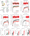
Fig. 1 |. Perturbation variance impairs sensorimotor adaptation.

a, Experiment setup (ff, force field). b, Fernandes and colleagues measured reach angle (bottom, $n=16$) during adaptation to variable rotations (top: s.d. = 0, 4 and 12° for zero-, low- and high-variances, respectively; mean = 30° for all). Participants exhibited residual errors (h, Fernandes; median error on last 48 trials; RMANOVA, $F(2,14)=17.8,P<0.001,{\eta }_p^2=0.54$). c, In Experiment 1, participants adapted to a zero-variance ($n=19$) or high-variance ($n=14$) perturbation (s.d. = 0 and 12° for zero- and high-variances; mean ^I = 30° for both). Residual error is shown in h, Experiment 1 (median of last 48 trials; $t\left(31\right)=4.24$, $P<0.001$, $d=1.49$, CI = [2.09, 5.96]). Retention was measured during an extended no-feedback period (No fb). d, In Experiment 2, we tested force field adaptation. Occasionally, we measured reaching forces on channel trials. Participants experienced a zero-variance ($n=12$) or high-variance ($n=13$) perturbation (top: s.d. = 0 and 6 N s m⁻¹ for zero- and high-variance; mean = 14 N s m⁻¹ for both). We computed an adaptation index on each channel trial (bottom). Residual error (h, Experiment 2, $t\left(23\right)=3.64$, $P=0.001$, $d=1.46$, CI = [0.08, 0.29]) is one minus the mean adaptation index on the last five error-clamp trials. e, In Experiment 3, we exposed participants to an extended period of rotations (160 epochs = 640 trials). Vertical dashed line indicates total number of rotation trials in Experiment 1. Participants adapted to a zero-variance ($n=10$) or high-variance ($n=10$) perturbation (top: s.d. = 0 and 12° for zero- and high-variance; mean = 30° for both). Mean residual error (h, Experiment 3, $t\left(18\right)=11.73$, $P<0.001$, $d=5.24$, CI = [5.74, 8.25]) was computed over last 50 epochs. To confirm that performance had reached a plateau, we measured slope of line fit to same period (g). Horizontal dashed lines show mean slope over first five epochs of perturbation. f, In Experiment 4, we adapted participants ($n=14$) to a zero-variance perturbation and then abruptly switched to a high-variance perturbation. Residual errors (h, Experiment 4, $t\left(26\right)=3.06$, $P=0.005$; $d=1.16$, CI = [0.94, 4.77]) were computed over last ten epochs of zero-variance period (f, horizontal line at ~25°) and high-variance period. g, Slope over first five (horizontal dashed lines) and last 50 epochs (points) in Experiment 3 (as in e). h, Residual errors in Fernandes and colleagues, and Experiments 1–4. Error bars are mean ± s.e.m.

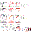
Fig. 2 |. Perturbation variance altered the total extent of implicit but not explicit adaptation.

a, In Experiment 5, participants ($n=11$) adapted to a zero-variance and high-variance rotation using delayed (~1 s) endpoint feedback (fb). Subjects adapted to both variance conditions (denoted Exposures 1 and 2) in a counterbalanced order. Explicit responses (solid lines, delay fb) in zero-variance and high-variance conditions are shown at left and right, respectively. Dashed lines show the same data for Experiment 1. Reach angles at top. Reaction times at bottom. b, Data from zero-variance and high-variance conditions are shown for Experiment 5. Residual error is shown at right over last ten rotation epochs. Left set of bars shows residual error over Exposures 1 and 2 (within-subject comparison, $t\left(10\right)=0.66$, $P=0.522$, $d=0.2$, 95% CI = [−1.95, 3.61]). Right set shows residual error only over Exposure 1 (between-subjects comparison, $t\left(9\right)=0.08$, $P=0.93$, $d=0.05$, 95% CI = [−6.11, 5.67]). c, Participants adapted to zero-variance ($n=13$) and high-variance ($n=12$) rotations under strict reaction time limits. Implicit responses (solid lines, ‘limit rxn’) in zero-variance and high-variance conditions shown at left and right, respectively. Data from Experiment 1 are shown in dashed lines. Reach angles at top. Reaction times at bottom. d, Comparison of zero-variance and high-variance learning in Experiment 6. Residual error over last ten rotation epochs shown at right ($t\left(23\right)=3.83$, $P<0.001$, $d=1.53$, 95% CI = [2.66, 8.93]). e, Learning is driven by implicit and explicit elements (left schematic, no instruction). Both components were measured in Experiment 7. Implicit measured by verbally instructing participants to move hand through the target without feedback (middle schematic, verbal instruction). Explicit measured by asking participants ($n=9$) to self-report aiming angle using visual landmarks (right schematic, self-report). f, Reach angles measured in Experiment 7. In grey region, implicit response is shown on verbal instruction trials. g, Column 1: residual errors on last ten rotations epochs ($t\left(16\right)=4.05$, $P<0.001$, $d=1.91$, 95% CI = [2.37, 7.6]). Column 2: implicit learning during verbal instruction ($t\left(16\right)=2.51$, $P=0.023$, $d=1.19$, 95% CI = [0.95, 11.21]). Column 3: explicit reach angle obtained from verbal instruction trials ($t\left(16\right)=0.41$, $P=0.69$, $d=0.19$, 95% CI = [−6.78, 4.59]). Column 4: explicit reach angle measured through self-report ($t\left(15\right)=0.77$, $P=0.45$, $d=0.37$, 95% CI = [−3.82, 8.15]). Error bars are mean ± s.e.m.

Fig. 3 |. Perturbation variance decreases error sensitivity, not decay rates.

a, State–space models of adaptation predict that learning will reach an asymptote when the amount of learning from an error exactly counterbalances the amount of forgetting that occurs between trials. The plot demonstrates the behaviour of such a model during adaptation to a perturbation of unit 1. The equation governing asymptotic learning is shown at bottom-right inset. b, According to the model, changes in asymptotic levels of performance can occur because of changes in forgetting (Possibility 1 schematic; a = 0.98 for low forgetting and 0.96 for high forgetting). c, Changes in asymptote can also be due to changes in error sensitivity (Possibility 2 schematic; b = 0.05 for low error sensitivity and 0.1 for high error sensitivity). d, To test Possibility 1, we measured the retention during error-free periods at the end of Experiment 1 (left; $n=19$ for zero-variance, $n=14$ for high-variance), Experiment 2 (middle; $n=12$ for zero-variance, n = 13 for high-variance) and Experiment 6 (right, $n=13$ for zero-variance, $n=12$ for high-variance). We normalized reach angle to the first trial in the no-feedback period. Each point on the x axis is a cycle of four trials. e, We measured the retention factor during error-free periods in each experiment depicted in d. We found no statistically significant difference in retention for zero-variance and high-variance groups (two-sample t-test, $t\left(81\right)=0.149$, $P=0.882$, $d=0.03$, 95% CI = [−0.006, 0.007]). f, To test Possibility 2, we measured error sensitivity in each experiment that terminated with an error-free period. Error sensitivity was greater for the zero-variance perturbation in every experiment (Experiment 1, $t\left(31\right)=3.35$, $P=0.002$, $d=1.18$, 95% CI = [0.088, 0.364]; Experiment 2, $t\left(23\right)=2.18$, $P=0.039$, $d=0.87$, 95% CI = [0.014, 0.5]; Experiment 4, $t\left(13\right)=3.41$, $P=0.005$, $d=0.91$, 95% CI = [0.10, 0.46]; Experiment 6, $t\left(23\right)=2.67$, $P=0.014$, $d=1.07$, 95% CI = [0.037, 0.293]). g, However, in Experiment 5 ($n=11$) we detected no statistically significant effect of perturbation variance on the rate of explicit learning ($t\left(10\right)=0.48$, $P=0.641$, $d=0.15$, 95% CI = [−0.396, 0.615]). The rate of learning was quantified by fitting exponential curves. Error bars are mean ± s.e.m.

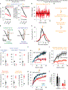
Fig. 4 |. Spatiotemporal variation in error sensitivity is predicted by error consistency.

a, Sorted pairs of movements based on error size. Error sensitivity (left) and error consistency (right) in error-size bins. Participants were combined across experiments with an implicit learning component and error-free period for retention measurements (Experiments 1, 4 and 6). Perturbation variability decreased error sensitivity (mixed-ANOVA, $F(1,84)=14.7,P<0.001,{\eta }_p^2=0.15$; Bonferroni-corrected t-tests, $t\left(71\right)=3.98$, $P<0.001$, $d=0.72$, 95% CI = [0.07, 0.28] for 5–14°; $t\left(71\right)=3.91$, $P<0.001$, $d=0.79$, 95% CI = [0.06, 0.21]I for 14–22°; $t\left(71\right)=1.44$, $P=0.53$, $d=0.32$, 95% CI = [−0.02, 0.08] for 22–30°) and error consistency (mixed-ANOVA, $F(1,84)=60.5,P<0.001,{\eta }_p^2=0.42$; Bonferroni-corrected t-tests, $t\left(71\right)=10.09$, $P<0.001$, $d=1.83$, 95% CI = [31.92, 51.58] for 5–14°; $t\left(71\right)=5.33$, $P<0.001$, $d=0.85$, 95% CI = [8.9, 28.05]I for 14–22°; $t\left(71\right)=2.0$, $P=0.16$, $d=0.37$, 95% CI = [−2.62, 11.54] for 22–30°) for small errors. b, We detected pairs of consistent errors (left, errors have same sign) and inconsistent errors (right, errors have opposite signs). Traces show example trajectories. c, Graphs (except bottom right) show fraction of inconsistent error trials. Variance increased inconsistency (Experiments 1, 3 and 7, $t\left(69\right)=2.74$, $P=0.008$, $d=0.65$, 95% CI = [0.02, 0.11]; Experiment 2, $t\left(23\right)=7.08$, $P<0.001$, $d=2.84$, 95% CI = [0.09, 0.16]; Experiment 4, $t\left(13\right)=9.35$, $P<0.001$, $d=2.50$, 95% CI = [0.16, 0.26]; Experiment 5, $t\left(10\right)=2.99$, $P=0.014$, $d=0.90$, 95% CI = [0.02, 0.12]; Experiment 6, $t\left(23\right)=2.09$, $P=0.048$, $d=0.84$, 95% CI = [0.001, 0.2]). Bottom right: variance increased s.d. of errors in Experiment 6 ($t\left(23\right)=3.86$, $P<0.001$, $d=1.55$, 95% CI = [6.98, 23.11]). d–g, Model predictions in Experiment 6. Perturbation variance (d) alters error distribution (e). Error sequences (collapsed in e) were placed into equation (1) to predict trial-by-trial error sensitivity. f, Mean predicted error sensitivity time course. Noisy curves show actual mean. Dashed blue lines show smoothed curve used in simulation. g, Implicit learning measured in Experiment 6 and simulated using predicted error sensitivity in f. h, Model predicts that perturbation variance impairs asymptotic learning: 1, perturbation variance decreases error consistency; 2, decreased consistency stunts error sensitivity growth; 3, stunted growth reduces asymptotic learning. i, Measured trial-to-trial implicit error sensitivity in Experiment 6. j, Change in error sensitivity from start to end of learning for measured behaviour in i (left bars in zero-variance and high-variance groups) and predicted behaviour in f (right bars in zero-variance and high-variance groups). Error sensitivity increased more in zero-variance condition ($t\left(23\right)=2.4$, $P=0.025$, $d=0.96$, 95% CI = [0.02, 0.32]). Error bars are mean ± s.e.m.

References

1. Albert ST & Shadmehr R The neural feedback response to error as a teaching signal for the motor learning system. J. Neurosci. 36, 4832–4845 (2016). - PMC - PubMed
1. Thoroughman KA & Shadmehr R Electromyographic correlates of learning an internal model of reaching movements. J. Neurosci. 19, 8573–8588 (1999). - PMC - PubMed
1. Franklin DW et al. CNS learns stable, accurate, and efficient movements using a simple algorithm. J. Neurosci. 28, 11165–11173 (2008). - PMC - PubMed
1. Shadmehr R, Brandt J & Corkin S Time-dependent motor memory processes in amnesic subjects. J. Neurophysiol. 80, 1590–1597 (1998). - PubMed
1. McDougle SD, Bond KM & Taylor JA Explicit and implicit processes constitute the fast and slow processes of sensorimotor learning. J. Neurosci. 35, 9568–9579 (2015). - PMC - PubMed
Publication types
LinkOut - more resources