TopoStats - A program for automated tracing of biomolecules from AFM images

Abstract

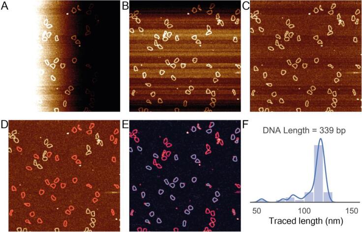
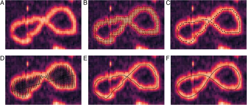
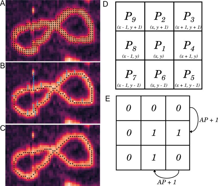
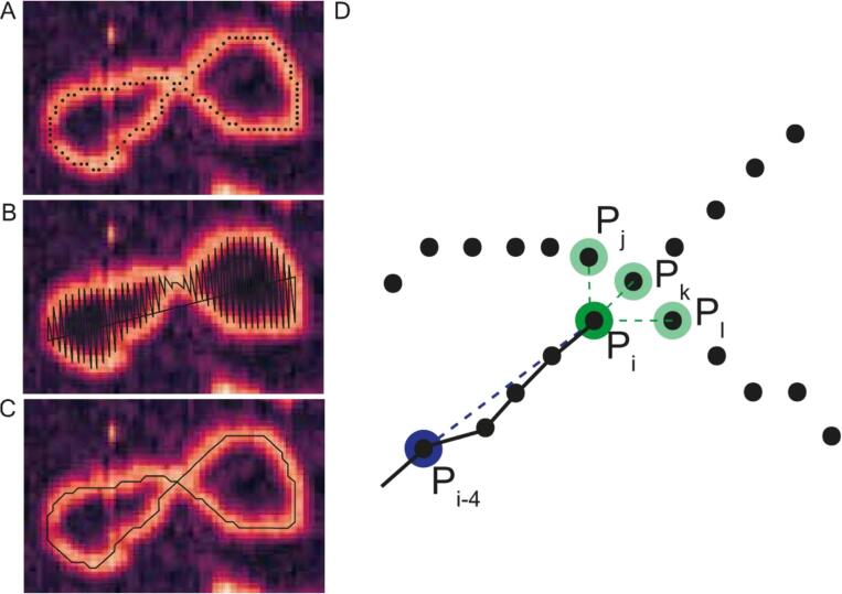
We present TopoStats, a Python toolkit for automated editing and analysis of Atomic Force Microscopy images. The program automates identification and tracing of individual molecules in circular and linear conformations without user input. TopoStats was able to identify and trace a range of molecules within AFM images, finding, on average, ~90% of all individual molecules and molecular assemblies within a wide field of view, and without the need for prior processing. DNA minicircles of varying size, DNA origami rings and pore forming proteins were identified and accurately traced with contour lengths of traces typically within 10 nm of the predicted contour length. TopoStats was also able to reliably identify and trace linear and enclosed circular molecules within a mixed population. The program is freely available via GitHub (https://github.com/afm-spm/TopoStats) and is intended to be modified and adapted for use if required.

Keywords: Atomic Force Microscopy (AFM); Biomolecular structure; DNA; Image analysis; Python scripting; Single-molecule imaging.

Fig. 1

Illustration of the sequential image processing and tracing steps undertaken by TopoStats for a raw AFM image of 339 base-pair DNA minicircles. A) The original Z-scanner positional values output by the AFM, note the severe image tilt occurring due to non-perfect alignment between the sample surface and the AFM tip. (B) The tilt corrected version of the AFM image shown in (A). (C) The z-axis offset corrected version of the image shown in B. (D) The fully corrected AFM image with the identified molecules shown in red. (E) The same AFM image with overlaid molecular traces in cyan (F) A histogram of the contour lengths (nm) for each measured DNA minicircle calculated from the traces shown in E. (For interpretation of the references to colour in this figure legend, the reader is referred to the web version of this article.)

Fig. 2

Representative image sequence showing the steps in the tracing process for an individual DNA molecule. (A) The original topographical image of a DNA minicircle. (B) The automatically generated Gwyddion grain (shown as black dots) overlaid on the DNA molecule. (C) The skeleton generated using our customised skeletonisation algorithm. Points in the skeleton are shown as black dots. (D) The cartesian coordinates for the skeleton are extracted using NumPy functions, note that the sequence of the coordinates leads to a nonsensical line trace connecting these coordinates (black line). (E) The corrected cartesian coordinates of the trace that now follows the trajectory of the underlying molecule. (F) The final smoothed trace generated by parametric splining.

Fig. 3

Schematic description of the skeletonisation function. (A) Example AFM image showing a DNA minicircle with the Gwyddion grain overlaid as black points. (B) A representative skeleton produced using the Zhang and Shuen approach in which branches (blue points) and redundant points (white points) can be seen within the trace. (C) The finalised skeleton with all branches and redundant points removed. (D) The naming convention for pixels within a 3x3 grid based on that used in Zhang and Shuen, 1984 as well as the reference cartesian coordinate positions for each pixel. (E) An example of a 3x3 pixel array evaluated for the (A)P1 rule. (For interpretation of the references to colour in this figure legend, the reader is referred to the web version of this article.)

Fig. 4

Schematic showing how the ordering process works. (A) An example image showing the pixelated binary skeleton. (B) The initial “disordered” trace in which coordinates are listed in ascending order based on the x-coordinate. Note how this trace does not follow the contours of the molecule. (C) The ordered trace that now follows the direction of the underlying molecule. (D) Diagrammatic representation of the angular search algorithm used to select the next point in the trace when multiple candidates are available. The point P_i is the reference point, and the reference angle is calculated using the vector between points P_i-4 and P_i. To distinguish between the candidate points, P_j, P_k and P_l, the angle between each candidate point and the reference point P_i-4 is calculated. The candidate point with the vector angle most similar to that between P_i and P_i-4 is accepted as the next point in the trace.

Fig. 5

(A) Schematic of the fit-improvement protocol. The grey bar represents the area that is interpolated to find the maximal height value, with the dashed red line representing the trace direction from which the perpendicular direction is determined. (B) Theoretical plot for a cross-section of height from a DNA molecule showing the original coordinate (P_intial, black point) and the corrected coordinate (P_optimal, blue point). (For interpretation of the references to colour in this figure legend, the reader is referred to the web version of this article.)

Fig. 6

Splining smoothes out the binary traces producing a more accurate trace. (A) The original poorly sampled trace, note its coarse sampling. (B) The splined trace which smoothly follows the contours of the underlying molecule.

Fig. 7

TopoStats tracing of a mixed set of images. For each dataset an (i) example AFM image is shown DNA traces overlaid in cyan and (ii) a histogram of the contour lengths. (A) 339 bp minicircles. (B) 251 bp minicircles. Blue stars represent the predicted contour lengths for each sample. Scale bars: 100 nm, vertical colour scale (inset colour bar in A): 3 nm. (For interpretation of the references to colour in this figure legend, the reader is referred to the web version of this article.)

Fig. 8

(A) Example traces (blue lines) for DNA minicircles of each length (left to right): 116 bp (i), 194 bp (ii), 256 bp (iii), 339 bp (iv), 357 bp (v), 398 bp (vi). Image widths: 80 nm, all images. Vertical scale: 6 nm (all images). (B) Kernel Density Estimate (KDE) plot showing the distributions for the measured contour lengths for each separate DNA minicircle population. Stars indicate the expected contour lengths for each sample. (C) Violin plot showing the distributions for the measured contour lengths for each separate DNA minicircle population. The median measured contour lengths are shown as white points, and correspond to 40, 59, 80, 113, 108, 118 nm, respectively. (D) Traced images from the 357 bp DNA minicircle population, note the distinct sizes of the minicircles in the top and bottom insets. (E) Traced images from the 398 bp DNA minicircle population. Scale bars: 200 nm, Vertical colour scale (inset colour bar in A): 3 nm. Images of individual DNA minicircles are 80 nm wide. (For interpretation of the references to colour in this figure legend, the reader is referred to the web version of this article.)

Fig. 9

AFM analysis of DNA minicircle conformation, identifying and tracing both linear and circular molecules automatically. A) AFM image of DNA minicircles, with individual molecules traced by TopoStats. Scale bar: 50 nm, vertical colour scale (inset colour bar in A): 3 nm. B) Violin plot showing the contour length distribution for both circular (length 58 ± 6 nm, N = 51) and linear (length 55 ± 14 nm, N = 76) molecules.

Fig. 10

TopoStats automated tracing of A) the membrane attack complex (MAC) protein pore, B) NuPOD DNA origami rings and C) the nuclear pore complex (NPC) (C). D) Traced lengths were plotted for both assemblies with contour lengths were determined as for the 60 ± 8 nm for the MAC and 166 ± 9 nm for DNA origami determined and 287 ± 21 nm for the NPC (N = 13, 456 and 15) respectively. Stars indicate the expected contour length. Scale bars are 200 nm, cropped images are 80 nm (A), 120 nm (B) and 200 nm (C) wide. Vertical colour scale (inset colour bar in A): 20 nm (A, B) 50 nm (C). Errors quoted are standard deviation.

References

1. Nievergelt A.P., Banterle N., Andany S.H., Gönczy P., Fantner G.E. High-speed photothermal off-resonance atomic force microscopy reveals assembly routes of centriolar scaffold protein SAS-6. Nat. Nanotechnol. 2018;13(8):696–701. doi: 10.1038/s41565-018-0149-4. - DOI - PubMed
1. Uchihashi T., Iino R., Ando T., Noji H. High-Speed Atomic Force Microscopy Reveals Rotary Catalysis of Rotorless F1-ATPase. Science. 2011;333(6043):755–758. doi: 10.1126/science.1205510. - DOI - PubMed
1. Pyne A., Thompson R., Leung C., Roy D., Hoogenboom B.W. Single-Molecule Reconstruction of Oligonucleotide Secondary Structure by Atomic Force Microscopy. Small. 2014;10(16):3257–3261. doi: 10.1002/smll.201400265. - DOI - PubMed
1. Uchihashi T., Watanabe Y.-H., Nakazaki Y., Yamasaki T., Watanabe H., Maruno T., Ishii K., Uchiyama S., Song C., Murata K., Iino R., Ando T. Dynamic structural states of ClpB involved in its disaggregation function. Nat. Commun. 2018;9(1) doi: 10.1038/s41467-018-04587-w. - DOI - PMC - PubMed
1. Kodera N., Yamamoto D., Ishikawa R., Ando T. Video imaging of walking myosin V by high-speed atomic force microscopy. Nature. 2010;468(7320):72–76. doi: 10.1038/nature09450. - DOI - PubMed
Publication types