Visualizing population structure with variational autoencoders

Abstract

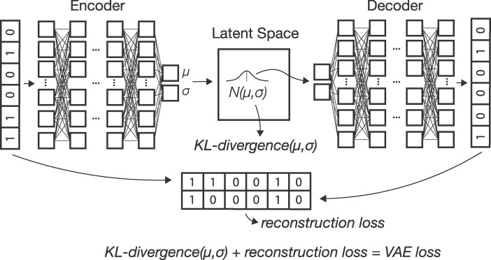
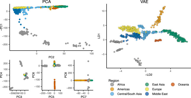
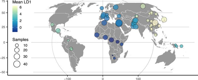
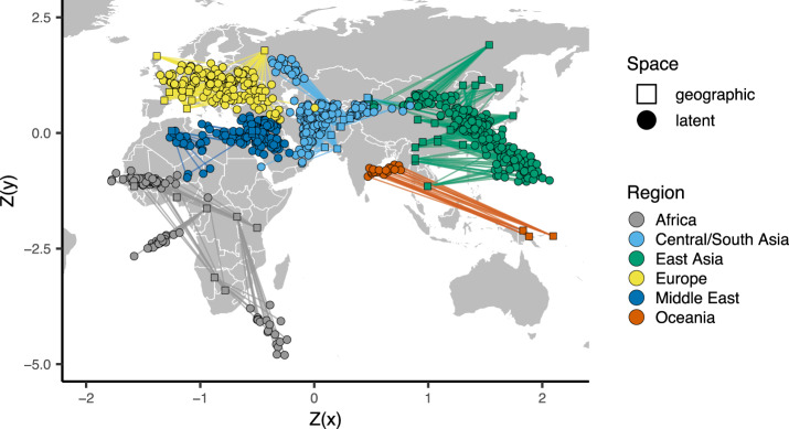
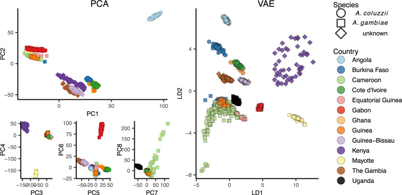
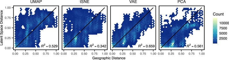
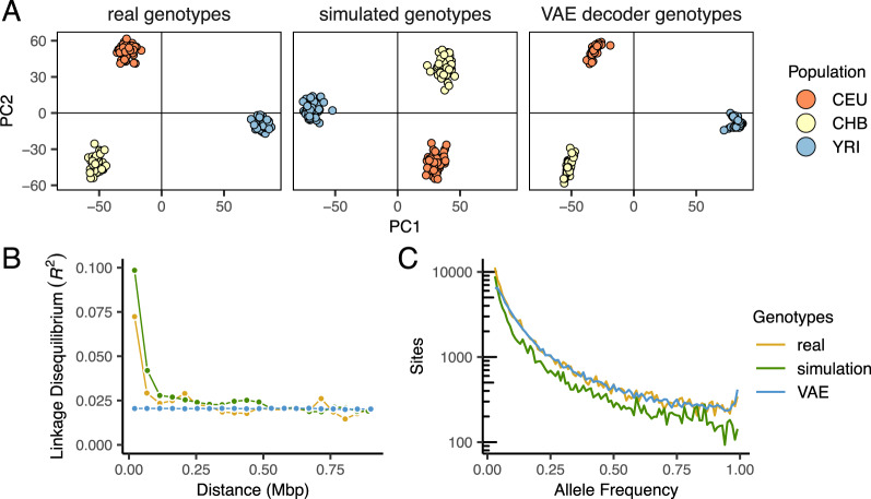
Dimensionality reduction is a common tool for visualization and inference of population structure from genotypes, but popular methods either return too many dimensions for easy plotting (PCA) or fail to preserve global geometry (t-SNE and UMAP). Here we explore the utility of variational autoencoders (VAEs)-generative machine learning models in which a pair of neural networks seek to first compress and then recreate the input data-for visualizing population genetic variation. VAEs incorporate nonlinear relationships, allow users to define the dimensionality of the latent space, and in our tests preserve global geometry better than t-SNE and UMAP. Our implementation, which we call popvae, is available as a command-line python program at github.com/kr-colab/popvae. The approach yields latent embeddings that capture subtle aspects of population structure in humans and Anopheles mosquitoes, and can generate artificial genotypes characteristic of a given sample or population.

Keywords: data visualization; deep learning; machine learning; neural network; pca; population genetics; population structure; variational autoencoder.

Figure 1

A schematic of the VAE architecture. Input allele counts are passed to an encoder network which outputs parameters describing a sample’s location as a multivariate normal in latent space. Samples from this distribution are then passed to a decoder network which generates a new genotype vector. The loss function used to update weights and biases of both networks is the sum of reconstruction error (from comparing true and generated genotypes) and KL divergence between sample latent distributions and $\mathcal{N}(0,1)$.

Figure 2

PCA axes 1–8 (left) and popvae run at default settings (right) for 100,000 random SNPs from chromosome 1 of the HGDP data. Axes are flipped to approximate geography.

Figure 3

HGDP population locations with color scaled to the mean latent coordinate of a 1D popvae latent space.

Figure 4

Comparing the VAE latent space with the geography of sampling localities in non-American HGDP samples (see Supplementary Figure S8 for a plot including the Americas). Circles show z-normalized sample locations in latent space and squares show the corresponding location in geographic space.

Figure 5

PCA (left) and VAE (right) run on 100,000 random SNPs from chromosome 3R of the AG1000G phase 2 data.

Figure 6

Latent spaces reflect inversion karyotypes at the 2La inversion in A. gambiae/coluzzii. (A) VAE latent spaces for AG1000G phase 2 samples from windows near the 2La inversion breakpoints, colored by species. (B) Multidimensional scaling values showing difference in the relative position of individuals in latent space across windows—high values reflect windows in which samples cluster by inversion karyotype, and low values by species.

Figure 7

VAE latent spaces and PCA run on two-population coalescent simulations with F_st varying from 0.0001 to 0.05. Points are colored by population. popvae was run with tuned hyperparameters and patience set to 500. See Supplementary Figure S12 for (much worse) performance with default settings.

Figure 8

Comparing pairwise distances in geographic and latent space for Eurasian human genotypes across four dimensionality reduction methods run at default settings. All distances are scaled to 0–1. Black lines show a 1:1 relationship.

Figure 9

Comparing real, VAE-generated, and simulated genotype matrices for three populations from the 1000 genomes project. The VAE decoder and coalescent simulation produce similar results in genotype PCA (A), but the VAE fails to reproduce the decay of LD with distance along the chromosome seen in real data (B). The site frequency spectrum is very similar for real and VAE-generated genotypes, but suffers from scaling issues in the coalescent simulation (C).

References

1. 1000 Genomes Project Consortium, et al.2015. A global reference for human genetic variation. Nature 526:68–74. - PMC - PubMed
1. Abadi M, Agarwal A, Barham P, Brevdo E, Chen Z, et al.2015. TensorFlow: large-scale machine learning on heterogeneous systems. Software available from tensorflow.org. (Accessed: 2020 October)
1. Adrion JR, Cole CB, Dukler N, Galloway JG, Gladstein AL, et al.2020a. A community-maintained standard library of population genetic models. eLife. 9:e54967. 10.7554/eLife.54967. - DOI - PMC - PubMed
1. Adrion JR, Galloway JG, Kern AD.. 2020b. Predicting the landscape of recombination using deep learning. Mole Biol Evol. 37:1790–1808. - PMC - PubMed
1. AG1000G Consortium. 2020. Genome variation and population structure among 1142 mosquitoes of the African malaria vector species anopheles gambiae and anopheles coluzzii. Genome Res. 30: 1533-1546. doi: 10.1101/gr.262790.120. - PMC - PubMed
Publication types
LinkOut - more resources