Computational analyses reveal spatial relationships between nuclear pore complexes and specific lamins

Abstract

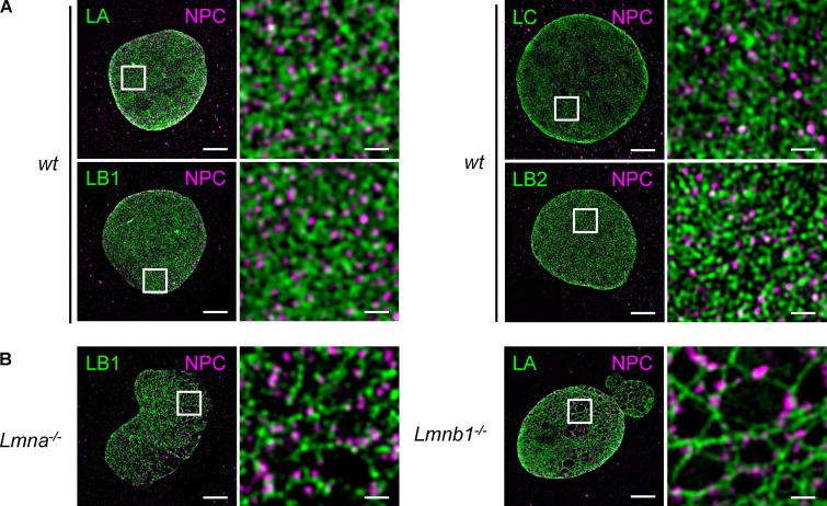
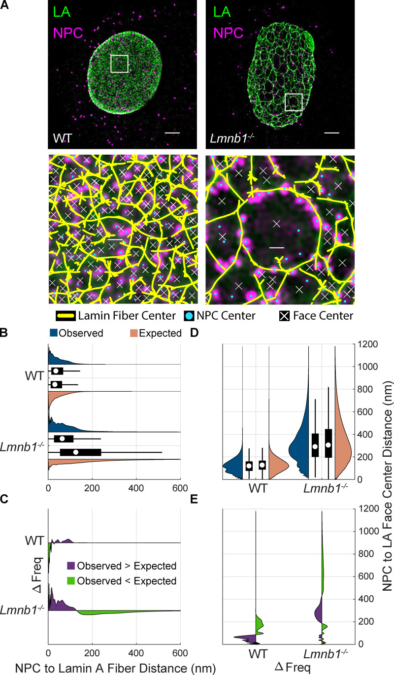
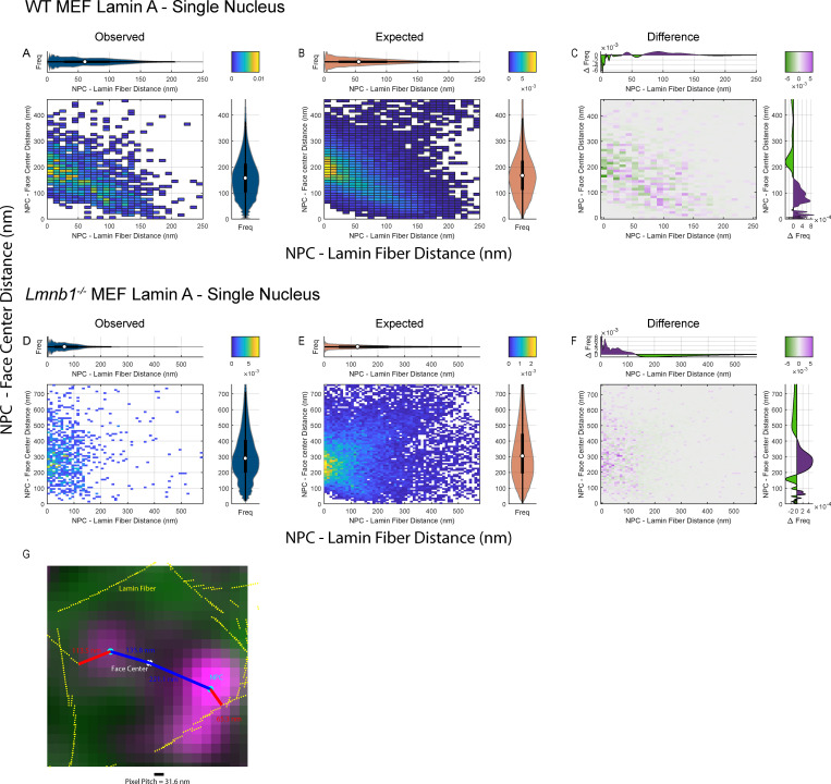
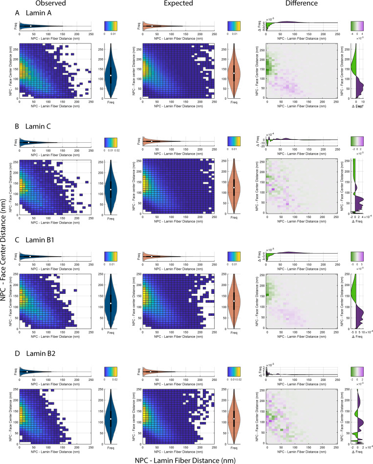
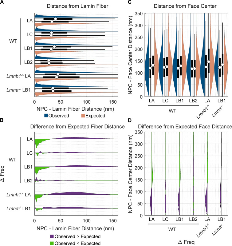
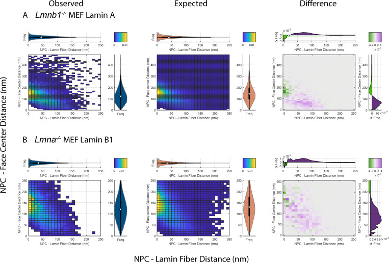
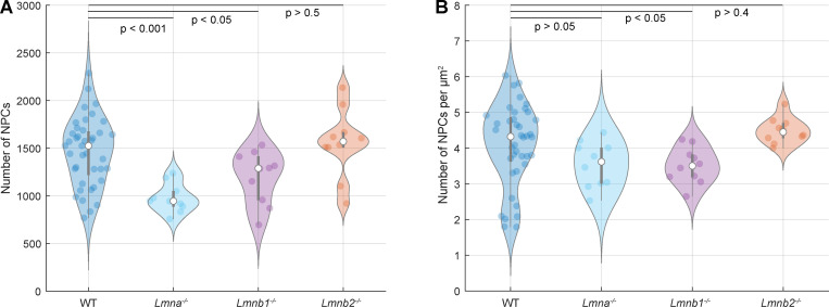
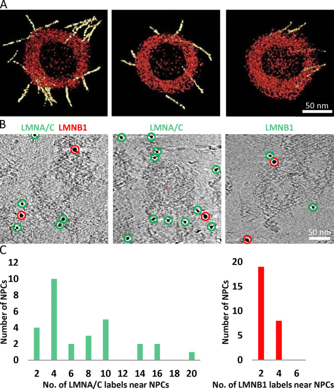
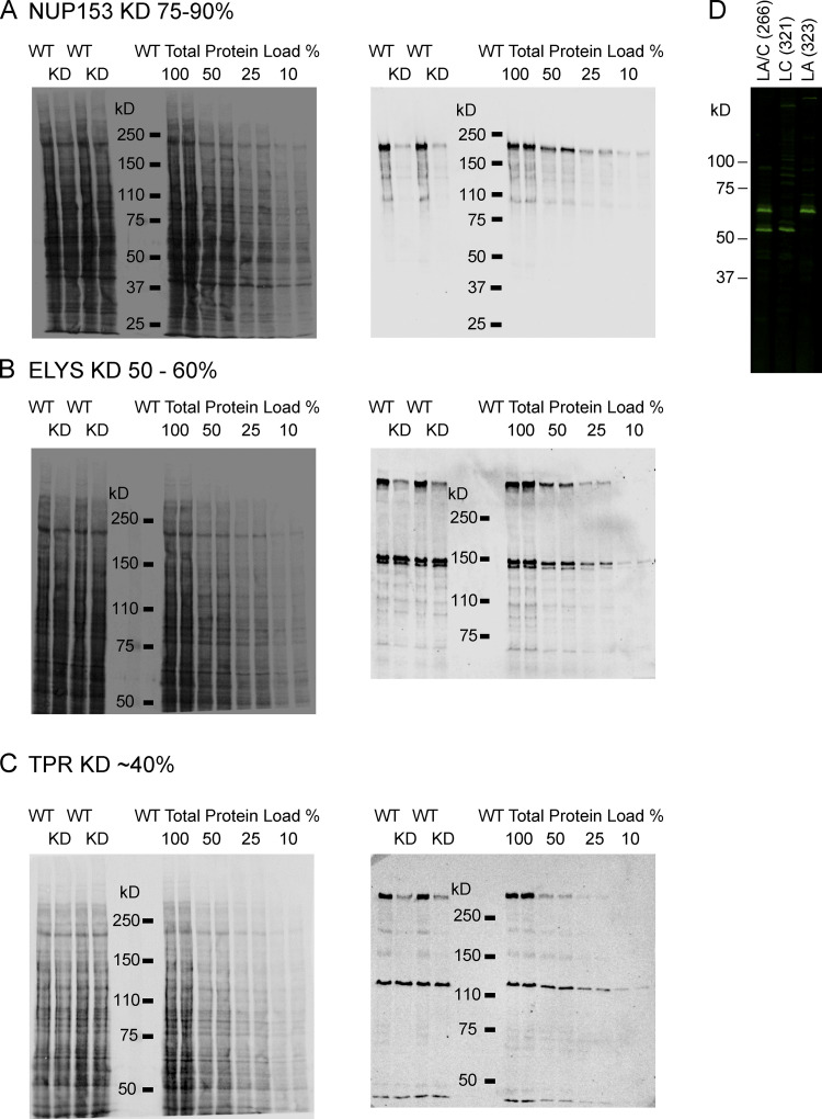
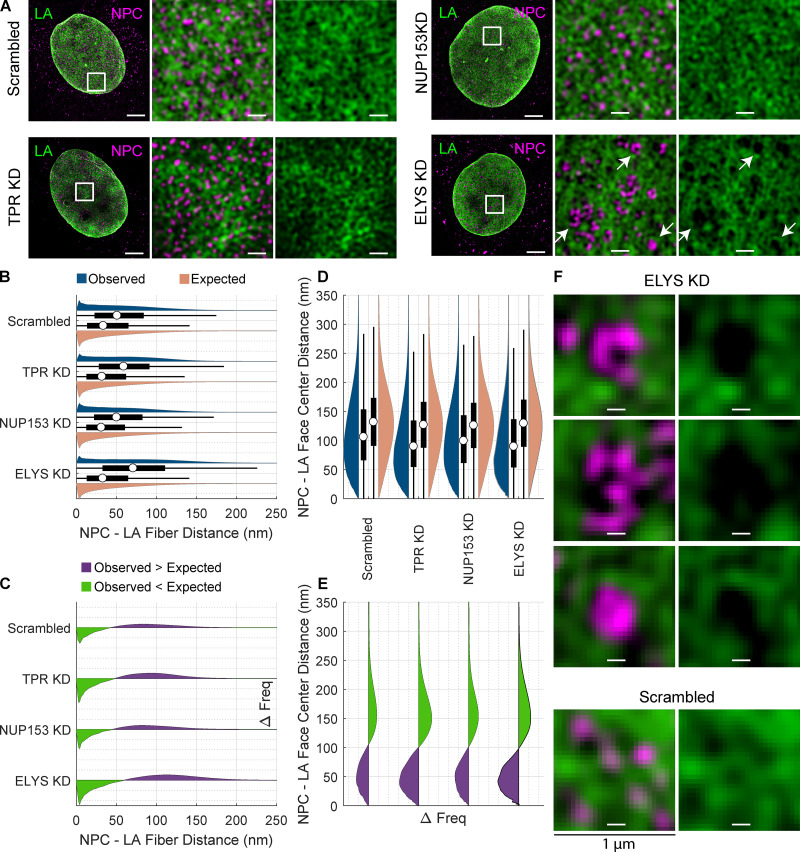
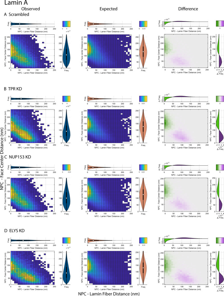
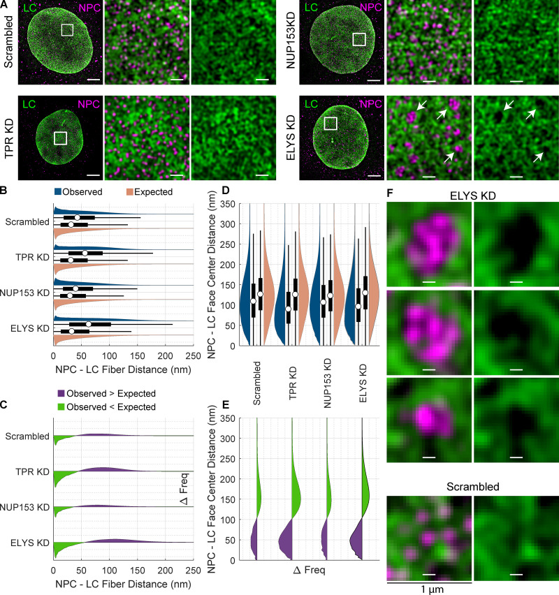
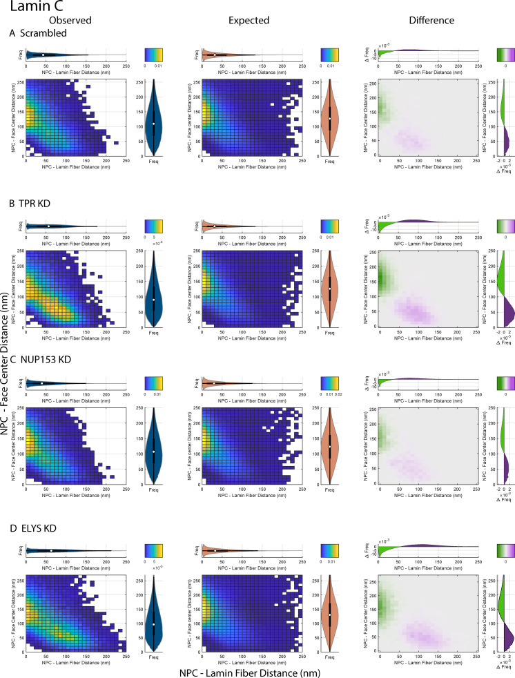
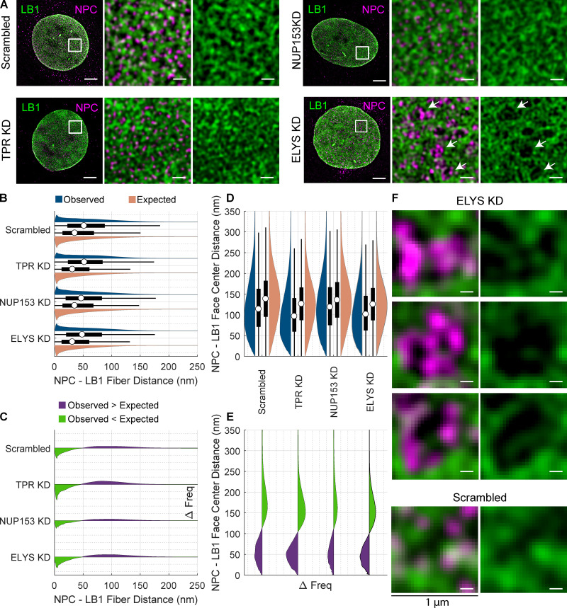
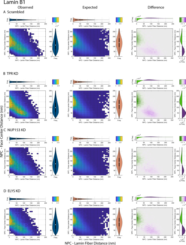
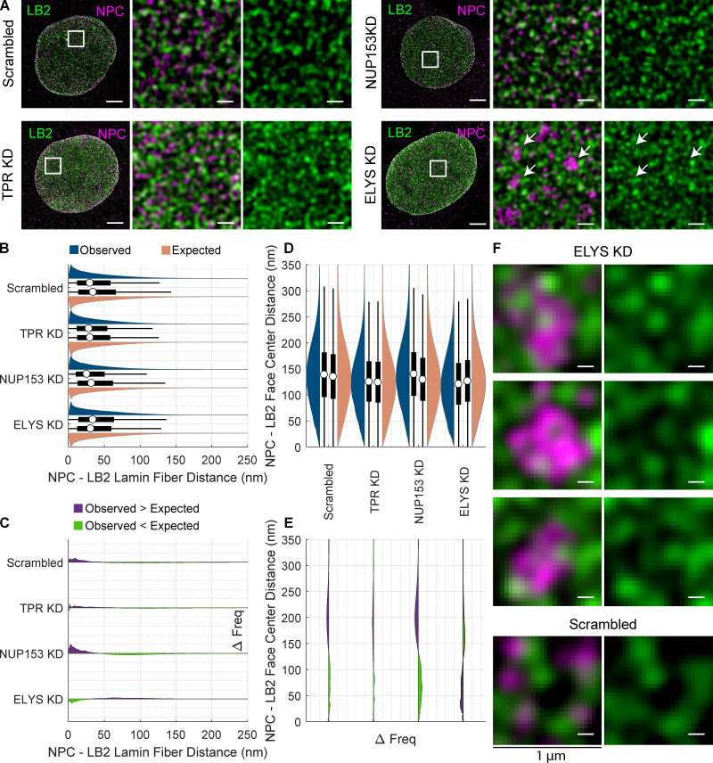
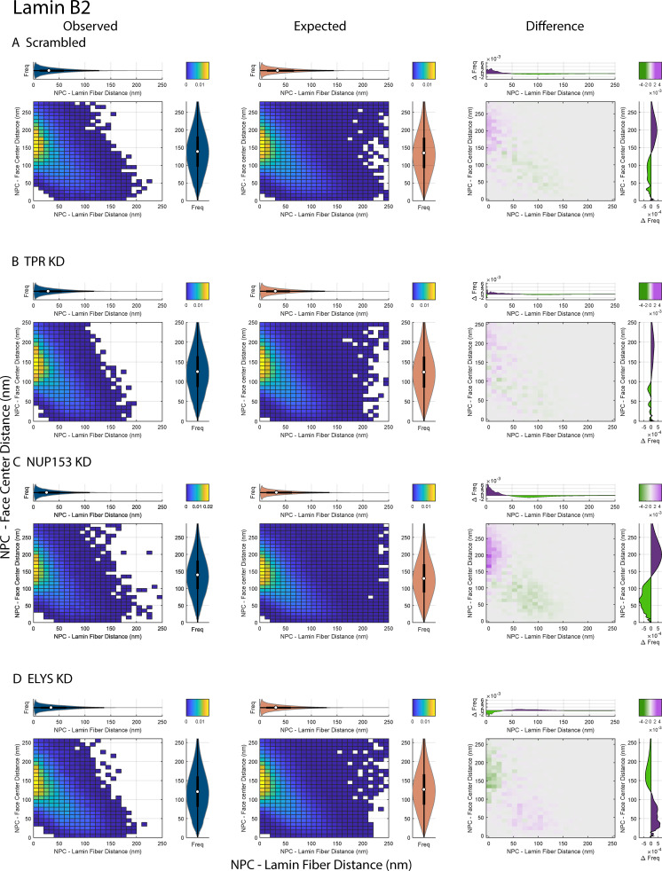
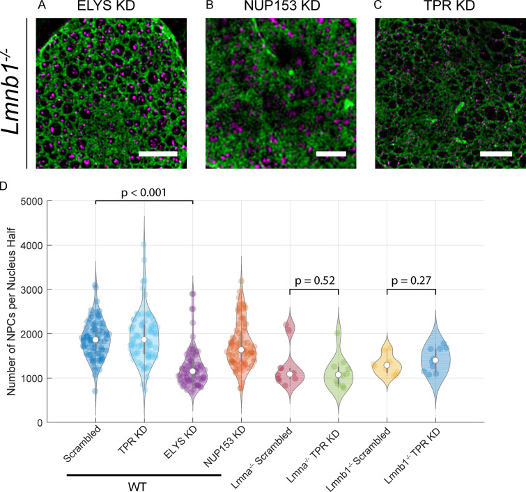
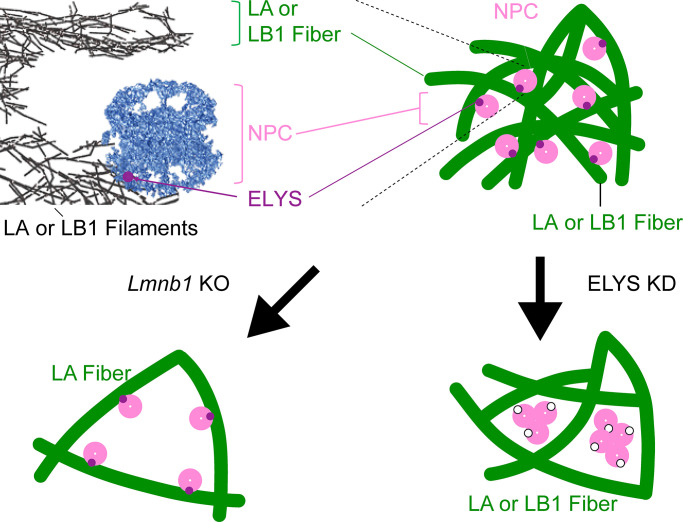
Nuclear lamin isoforms form fibrous meshworks associated with nuclear pore complexes (NPCs). Using datasets prepared from subpixel and segmentation analyses of 3D-structured illumination microscopy images of WT and lamin isoform knockout mouse embryo fibroblasts, we determined with high precision the spatial association of NPCs with specific lamin isoform fibers. These relationships are retained in the enlarged lamin meshworks of Lmna-/- and Lmnb1-/- fibroblast nuclei. Cryo-ET observations reveal that the lamin filaments composing the fibers contact the nucleoplasmic ring of NPCs. Knockdown of the ring-associated nucleoporin ELYS induces NPC clusters that exclude lamin A/C fibers but include LB1 and LB2 fibers. Knockdown of the nucleoporin TPR or NUP153 alters the arrangement of lamin fibers and NPCs. Evidence that the number of NPCs is regulated by specific lamin isoforms is presented. Overall the results demonstrate that lamin isoforms and nucleoporins act together to maintain the normal organization of lamin meshworks and NPCs within the nuclear envelope.

Figure 1.

NPCs are arranged along LA and LB1 fibers in enlarged lamin meshworks. (A and B) Colabeling of lamins and NPCs in WT and lamin KO MEF nuclei using indirect immunofluorescence with a pair of specific antibodies against each lamin isoform (LA, LB1, LB2, or LC) and the FXFG-repeat nucleoporins. (A) WT MEF nuclei colabeled with the indicated lamin isoform and FXFG-repeated nucleoporins. (B) Nuclei of Lmna^−/− (left pair) and Lmnb1^−/− (right pair) MEFs. The indicated areas with white squares are enlarged approximately eightfold along each edge and are displayed on the right side of each pair of images. Scale bar = 5 µm (full), 625 nm (inset).

Figure 2.

Computational image analysis reveals that NPCs are closely associated with LA fibers. (A–E) Each plot reflects a single nucleus and is meant to illustrate the analysis process rather than show a representative distribution as in later figures. (A) Immunofluoresence images labeling LA (green) and NPCs (magenta) of WT and Lmnb1^−/− MEF nuclei as in Fig. 1 were subjected to computational image analysis. White boxes in the top row are magnified eight times along each edge. The centers of LA fibers (yellow lines), NPCs (cyan dots), and faces (white Xs) were segmented to subpixel precision (Kittisopikul et al., 2020); Materials and methods). Scale bar = 5 µm (full), 625 nm (inset). (B) Paired violin and box plots of NPC to LA fiber distances for the nuclei in A. The violin (blue) and box plots on top represent the observed distance distributions. The violin (red) and box plots on bottom represent the expected distance distributions under the null hypothesis. The white circle indicates the median. The thick black bar indicates the interquartile range (IQR). The black whiskers indicate 1.5 times the IQR. (C) Frequency (Freq) difference plot of observed minus expected LA fiber to NPC distances. The green portion below the line indicates where the observed frequency is less than expected. The purple portion above the line indicates where the observed frequency is greater than expected. (D) NPC to LA face center distances displayed as in B, rotated 90° counterclockwise. (E) Frequency difference plot of NPC to LA face center distances, displayed as in C, rotated 90° counterclockwise.

Figure S1.

Bivariate histograms of LA fiber–NPC and face center–NPC distances in single nuclei; illustration of distances. (A) Observed bivariate histogram of NPC to LA face center distances versus NPC to LA fiber distances of a single WT MEF LA nucleus shown in Fig. 2 A. (B) Expected bivariate histogram of NPC to LA face center distances versus NPC to LA fiber distances of a single WT MEF nucleus under the null hypothesis. (C) Difference between the observed and expected distance distributions with purple indicating where the observed exceeds the expected frequency (Freq) and green showing when the observed frequency is less than the expected frequency. (D–F) Same as A–C except for the single Lmnb1^−/− nucleus shown in Fig. 2 A. Marginal violin plots and box plots of the distances correspond with the half-violin plot counterparts of the same orientation and color as in Fig. 2 B. (G) Zoomed-in plot showing the NPC to LA fiber (red) and NPC to LA face center (blue) distances measured. Other colors correspond with those as in Fig. 2 B.

Figure S2.

Bivariate histograms of WT MEFs of NPC to face-versus-fiber distances show lamin isoform-dependent 2D distribution patterns. (A) First row shows a bivariate distribution of NPC to LA fiber and face center distances in WT MEFs. (B) Second row shows bivariate distributions of NPC to LC fiber and face center distances. (C) Third row shows bivariate distributions of NPC to LB1 distances. (D) Fourth row shows bivariate distributions of NPC to LB2 distances. (A–D) First column represents the observed bivariate distribution. Second column represents the expected bivariate distribution. Third column represents the difference between expected and observed. Difference between the observed and expected distance distributions with purple indicating where the observed exceeds the expected frequency (Freq) and green showing when the observed frequency is less than the expected frequency. Marginal violin plots and box plots of the distances correspond with the half-violin plot counterparts of the same orientation and color as in Fig. 3 B. Each violin or box plot represents 10 cells with the number of NPCs detailed in Table 1.

Figure 3.

Quantitative analysis of lamin–NPC distances over many nuclei reveals NPCs are offset from the center of LA and LB1 fibers in WT, Lmna^−/−, and Lmnb1^−/− MEFs by 20–30 nm. (A) Paired violin and box plots of NPC to lamin fiber distances. The violin (blue) and box plots on top represent the observed distance distributions. The violin (red) and box plots on bottom represent the expected distance distributions under the null hypothesis. The white circles indicate the medians. The thick black bar indicates the interquartile range (IQR). The black whiskers indicate 1.5 times the IQR. (B) Frequency (Freq) difference plots of observed minus expected lamin fiber to NPC distances. The green portion below the line indicates where the observed frequency is less than expected. The purple portion above the line indicates where the observed frequency is greater than expected. (C) NPC to lamin face center distances displayed as in A, rotated 90° counterclockwise. (D) Frequency difference plot of NPC to lamin face center distances, displayed as in C, rotated 90° counterclockwise. Each violin or box plot represents 10 cells with the number of NPCs detailed in Table 1.

Figure S3.

Bivariate histograms of Lmnb1^−/− and Lmna^−/− MEFs. (A) First row corresponds to the NPC to LA fiber and face center distances in Lmnb1^−/− MEFs. (B) Second row shows NPC to LB1 fiber and face center distances in Lmna^−/− MEFs. Columns are as in Fig. S2. Each violin or box plot represents 10 cells with the number of NPCs detailed in Table 1. Freq, frequency.

Figure S4.

Violin plots comparing the number of NPCs detected in WT, Lmna^−/−, Lmnb1^−/−, and Lmnb2^−/− MEFs. (A and B) Number of NPCs per nucleus (A) and NPC density for WT, Lmna^−/−, Lmnb1^−/−, and Lmnb2^−/− MEFs (B). The WT category is comprised of 10 cells pooled from the cells counted in the first four rows of Table 1 and Table 2, consisting of cells of WT genotype and stained with antibodies against the four lamin isoforms. The Lmna^−/− category consists of 10 cells corresponding to the sixth row of Table 1 and Table 2. The Lmnb1^−/− category consists of 10 cells corresponding to the fifth row of Table 1 and Table 2. The Lmnb2^−/− category consists of 10 cells. The white circles indicate the medians. The thick gray bar indicates the interquartile range (IQR). The gray whiskers indicate 1.5 times the IQR. Each colored circle corresponds to a single cell. The Mann-Whitney U test was used to compare distributions and determine P values as described in the Materials and methods.

Figure 4.

Cryo-ET showing LA/LC and LB1 filament contacts with the nucleoplasmic ring. (A) Lamin filaments (yellow) interact with NPCs (red) as seen by surface rendering representations of cryo-subtomograms. (B) Gold labeling of lamin filaments observed by cryo-ET. The position of LA/LC labels (green) and LB1 labels (red) are indicated. Double labeling (left) or labeling of individual lamin isoforms was analyzed and presented as histograms. The unmarked gold particles (middle, right) are fiducial markers. (C) A total number of 214 LA/LC labels and 70 LB1 labels were detected around 47 nucleoplasmic rings.

Figure S5.

Western blots of ELYS, NUP153, and TPR siRNA KD experiments and of anti-LC specificity. (A–C) siRNA KDs were performed and quantified as described in Materials and methods. The panels on the left are the total protein stains of the immunoblots with each sample loaded in duplicate. The panels on the right are the immunoblots for each antibody NUP153 (A), ELYS (B), and TPR (C). The degree of KD for each protein was determined by quantifying the average intensity of each duplicate after correction for protein load and comparison to the dilution series of the total protein load from WT cells. (D) Whole cell lysates of WT MEFs in Laemmli sample buffer were resolved by SDS-PAGE (6 ×10⁴ cells/lane); immunoblotted by anti-LA/LC (266) 1:1,000; anti-LC (321) 1:500; and anti-LA (323) 1:1,000 primary antibodies along with anti-rabbit secondary antibody (LICOR; IRDye 800CW) and visualized using Odyssey Fc at 800 nm.

Figure 5.

Co-distribution of LA and NPC components after siRNA transfection shows enlarged LA meshworks filled with NPC clusters upon ELYS KD. (A) Immunofluorescence images of LA (green) and NPCs (magenta) following KDs of TPR, NUP153, ELYS, and scramble control. Note the clustering of NPCs in the ELYS KD. Area of white box (left) is shown merged (center) and just lamin (right). White arrows indicate areas of NPC clustering. Scale bar = 5 µm (full), 625 nm (inset). (B) Paired violin and box plots of NPC center to LA fiber center distances. The violin (blue) and box plots represent the observed distance distributions. The violin (red) and box plots on bottom represent the expected distance distributions under the null hypothesis. The white circle indicates the median. The thick black bar indicates the interquartile range (IQR). The black whiskers indicate 1.5 times the IQR. (C) Frequency (Freq) difference plots of observed minus expected LA fiber to NPC distances for the KD series. The green portion below the line indicates where the observed frequency is less than expected. The purple portion above the line indicates where the observed frequency is greater than expected. (D) NPC center to LA face center distances displayed as in B, rotated 90° counterclockwise. (E) Frequency difference plot of NPC to LA face center distances, displayed as in C, rotated 90° counterclockwise. (F) 1-µm² areas around NPC clusters formed after scramble treatment or ELYS KD indicated by white arrows in A shown merged (left) and just lamin (right). Each violin or box plot represents 20 cells with the number of NPCs detailed in Table 3. Scale bar = 150 nm.

Figure S6.

Bivariate histograms of LA fiber–NPC and face center–NPC distances. (A) First row shows a bivariate distribution of NPC to LA fiber and face center distances in WT MEFs after treatment with scramble siRNA. (B) Second row shows the same with siRNA KD of TPR. (C) Third row shows the same with siRNA KD of NUP153. (D) Fourth row shows the same with siRNA KD of ELYS. (A–D) First column represents the observed bivariate distribution. Second column represents the expected bivariate distribution. Third column represents the difference between expected and observed. Difference between the observed and expected distance distributions with purple indicating where the observed exceeds the expected frequency (Freq) and green showing when the observed frequency is less than the expected frequency. Marginal violin plots and box plots of the distances correspond with the half-violin plot counterparts of the same orientation and color as in Fig. 5, B–E. Each violin or box plot represents 20 cells with the number of NPCs detailed in Table 3.

Figure 6.

Co-distribution of LC and NPC components after siRNA transfection shows enlarged LC meshwork filled with NPC clusters upon ELYS KD. (A) Double-label immunofluoresence images of LC (green) and NPCs (magenta) following KDs of TPR, NUP153, ELYS, and scramble control. Area of white box (left) is shown merged (center) and just lamin (right). White arrows indicate areas of NPC clustering. Scale bar = 5 µm (full), 625 nm (inset). (B) Paired violin and box plots of NPC center to LC fiber center distances. The violin (blue) and box plots on top represent the observed distance distributions. The violin (red) and box plots on bottom represent the expected distance distributions under the null hypothesis. The white circle indicates the median. The thick black bar indicates the interquartile range (IQR). The black whiskers indicate 1.5 times the IQR. (C) Frequency (Freq) difference plots of observed minus expected LC fiber to NPC distances for the KD series. The green portion below the line indicates where the observed frequency is less than expected. The purple portion above the line indicates where the observed frequency is greater than expected. (D) NPC center to LC face center distances displayed as in B, rotated 90° counterclockwise. (E) Frequency difference plot of NPC center to LC face center distances, displayed as in C, rotated 90° counterclockwise. (F) 1-µm² areas around NPC clusters formed after scramble treatment or ELYS KD indicated by white arrows in A shown merged (left) and just lamin (right). Each violin or box plot represents 20 cells with the number of NPCs detailed in Table 3. Scale bar = 150 nm.

Figure S7.

Bivariate histograms of LC fiber–NPC and face center–NPC distances. (A) First row shows a bivariate distribution of NPC to LC fiber and face center distances in WT MEFs after treatment with scramble siRNA. (B) Second row shows the same with siRNA KD of TPR. (C) Third row shows the same with siRNA KD of NUP153. (D) Fourth row shows the same with siRNA KD of ELYS. (A–D) First column represents the observed bivariate distribution. Second column represents the expected bivariate distribution. Third column represents the difference between expected and observed. Difference between the observed and expected distance distributions with purple indicating where the observed exceeds the expected frequency and green showing when the observed frequency (Freq) is less than the expected frequency. Marginal violin plots and box plots of the distances correspond with the half-violin plot counterparts of the same orientation and color as in Fig. 6, B–E. Each violin or box plot represents 20 cells with the number of NPCs detailed in Table 3.

Figure 7.

Co-distribution of LB1 and NPCs after siRNA transfection reveals LB1 fibers within NPC clusters upon ELYS KD. (A) Double-label immunofluoresence images of LB1 (green) and NPCs (magenta) following KDs of TPR, NUP153, ELYS, and scramble control. Area of white box (left) is shown merged (center) and just lamin (right). White arrows indicate areas of NPC clustering. Scale bar = 5 µm (full), 625 nm (inset). (B) Paired violin and box plots of NPC center to LB1 fiber center distances. The violin (blue) and box plots on top represent the observed distance distributions. The violin (red) and box plots on bottom represent the expected distance distributions under the null hypothesis. The white circle indicates the median. The thick black bar indicates the interquartile range (IQR). The black whiskers indicate 1.5 times the IQR. (C) Frequency (Freq) difference plot of observed minus expected LB1 fiber to NPC center distances for the KD series. The green portion below the line indicates where the observed frequency is less than expected. The purple portion above the line indicates where the observed frequency is greater than expected. (D) NPC center to LB1 face center distances displayed as in B, rotated 90° counterclockwise. (E) Frequency difference plot of NPC to LB1 face center distances, displayed as in C, rotated 90° counterclockwise. (F) 1-µm² areas around NPC clusters formed after scramble treatment or ELYS KD indicated by white arrows in A shown merged (left) and just lamin (right). Each violin or box plot represents 20 cells with the number of NPCs detailed in Table 3. Scale bar = 150 nm.

Figure S8.

Bivariate histograms of LB1 fiber–NPC and face center–NPC distances. (A) First row shows a bivariate distribution of NPC to LB1 fiber and face center distances in WT MEFs after treatment with scramble siRNA. (B) Second row shows the same with siRNA KD of TPR. (C) Third row shows the same with siRNA KD of NUP153. (D) Fourth row shows the same with siRNA KD of ELYS. (A–D) First column represents the observed bivariate distribution. Second column represents the expected bivariate distribution. Third column represents the difference between expected and observed. Difference between the observed and expected distance distributions with purple indicating where the observed exceeds the expected frequency (Freq) and green showing when the observed frequency is less than the expected frequency. Marginal violin plots and box plots of the distances correspond with the half-violin plot counterparts of the same orientation and color as in panels B–E of Fig. 7. Each violin or box plot represents 20 cells with the number of NPCs detailed in Table 3.

Figure 8.

Co-distribution of LB2 and NPCs after siRNA transfection does not show enlarged faces around NPC clusters upon ELYS KD. (A) Immunofluorescence images of LB2 (green) and NPCs (magenta) following KDs of TPR, NUP153, ELYS, and scramble control. Area of white box (left) is shown merged (center) and just lamin (right). White arrows indicate areas of NPC clustering. Scale bar = 5 µm (full), 625 nm (inset). (B) Paired violin and box plots of NPC center to LB2 fiber center distances. The violin (blue) and box plots on top represent the observed distance distributions. The violin (red) and box plots on bottom represent the expected distance distributions under the null hypothesis. The white circle indicates the median. The thick black bar indicates the interquartile range (IQR). The black whiskers indicate 1.5 times the IQR. (C) Frequency (Freq) difference plot of observed minus expected LB2 fiber center to NPC center distances. The green portion below the line indicates where the observed frequency is less than expected. The purple portion above the line indicates where the observed frequency is greater than expected. (D) NPC center to LB2 face center distances displayed as in B, rotated 90° counterclockwise. (E) Frequency difference plot of NPC to LB2 face center distances, displayed as in C, rotated 90° counterclockwise. (F) 1-µm² areas around NPC clusters formed after scramble treatment or ELYS KD indicated by white arrows in A shown merged (left) and just lamin (right). Each violin or box plot represents 20 cells with the number of NPCs detailed in Table 3. Scale bar = 150 nm.

Figure S9.

Bivariate histograms of LB2 fiber–NPC and face center–NPC distances. (A) First row shows a bivariate distribution of NPC to LB2 fiber and face center distances in WT MEFs after treatment with scramble siRNA. (B) Second row shows the same with siRNA KD of TPR. (C) Third row shows the same with siRNA KD of NUP153. (D) Fourth row shows the same with siRNA KD of ELYS. (A–D) First column represents the observed bivariate distribution. Second column represents the expected bivariate distribution. Third column represents the difference between expected and observed. Difference between the observed and expected distance distributions with purple indicating where the observed exceeds the expected frequency and green showing when the observed frequency is less than the expected frequency. Marginal violin plots and box plots of the distances correspond with the half-violin plot counterparts of the same orientation and color as in panels B–E of Fig. 8. Each violin or box plot represents 20 cells with the number of NPCs detailed in Table 3.

Figure S10.

Effect of ELYS, NUP153, and TPR KD in Lmnb1^−/− and Lmna^−/− MEFs. (A–C) Immunofluoresence images of Lmnb1^−/− MEFs ELYS KD (A), NUP153 KD (B), TPR KD (C) with LA (green) and NPCs (magenta) labeled. (D) Number of NPCs per MEF nuclei in a single focal plane in WT MEFs after ELYS (80 cells), NUP153 (80 cells), and TPR (80 cells) KD; in Lmna^−/− MEFs after TPR KD (10 cells); and in Lmnb1^−/− MEFs after TPR KD (10 cells) in comparison to scrambled siRNA (80 WT MEFs, 10 Lmna^−/− MEFs, 10 Lmnb1^−/− MEFs). The white circles indicate the medians. The thick gray bar indicates the interquartile range (IQR). The gray whiskers indicate 1.5 times the IQR. Each colored circle represents a single cell. The Mann-Whitney U test was used to compare the distributions as described in the Materials and methods. Scale bar = 10 µm.

Figure 9.

Schema of lamin-NPC interactions. Top left: structure of LA or LB1 fibers consisting of individual filaments and an NPC as seen by cryo-ET. Top right: NPCs associating next to LA or B1 fibers at the resolution of structured illumination light microscopy. Bottom left: knocking out LB1 results in enlarged faces where NPCs adhere to LA fibers. Bottom right: knocking down ELYS results in enlarged faces containing clusters of NPCs missing ELYS (see Discussion).

References

1. Aebi, U., Cohn J., Buhle L., and Gerace L.. 1986. The nuclear lamina is a meshwork of intermediate-type filaments. Nature. 323:560–564. 10.1038/323560a0 - DOI - PubMed
1. Al-Haboubi, T., Shumaker D.K., Köser J., Wehnert M., and Fahrenkrog B.. 2011. Distinct association of the nuclear pore protein Nup153 with A- and B-type lamins. Nucleus. 2:500–509. 10.4161/nucl.2.5.17913 - DOI - PubMed
1. Beck, M., and Hurt E.. 2017. The nuclear pore complex: understanding its function through structural insight. Nat. Rev. Mol. Cell Biol. 18:73–89. 10.1038/nrm.2016.147 - DOI - PubMed
1. Broers, J.L., Machiels B.M., van Eys G.J., Kuijpers H.J., Manders E.M., van Driel R., and Ramaekers F.C.. 1999. Dynamics of the nuclear lamina as monitored by GFP-tagged A-type lamins. J. Cell Sci. 112:3463–3475 https://jcs.biologists.org/content/112/20/3463. - PubMed
1. Burke, B., and Stewart C.L.. 2014. Functional Architecture of the Cell’s Nucleus in Development, Aging, and Disease. In Current Topics in Developmental Biology. Elsevier, San Diego. 1–52., 10.1016/B978-0-12-397920-9.00006-8 - DOI - PubMed
Publication types