. 2021 Mar;53(3):367-378.
doi: 10.1038/s41588-021-00784-4. Epub 2021 Feb 11.

Liquid chromatin Hi-C characterizes compartment-dependent chromatin interaction dynamics

Affiliations

Liquid chromatin Hi-C characterizes compartment-dependent chromatin interaction dynamics

Houda Belaghzal et al. Nat Genet. 2021 Mar.

Abstract

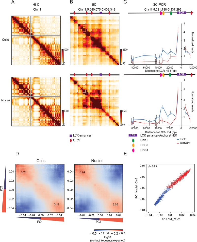
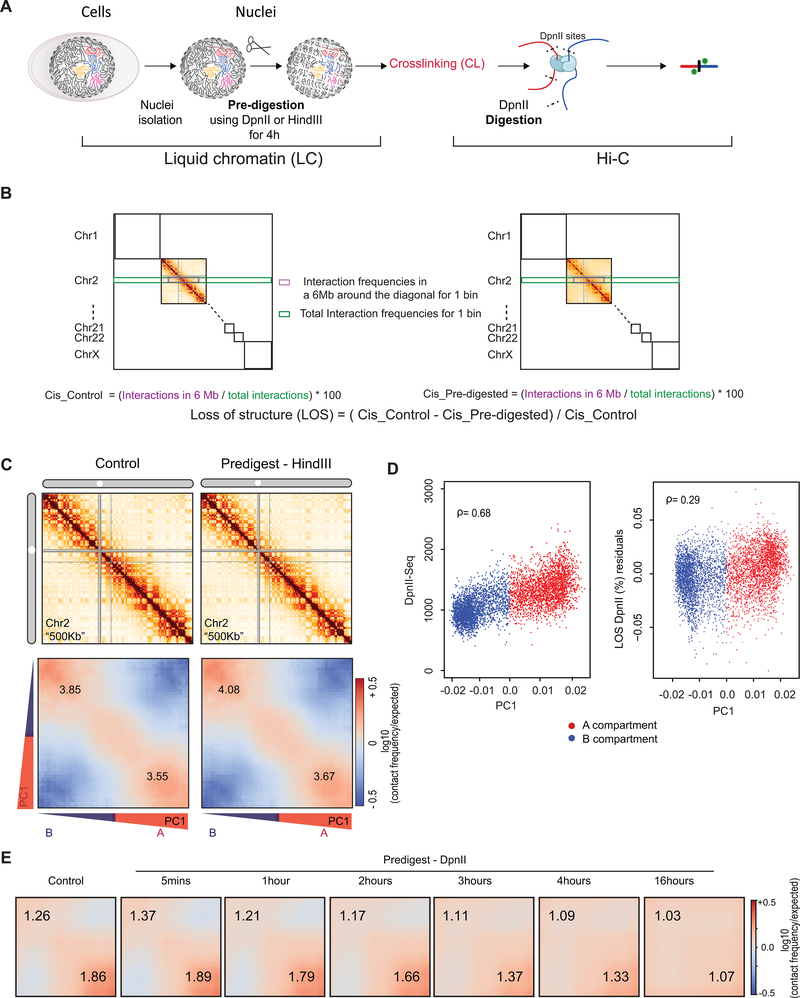
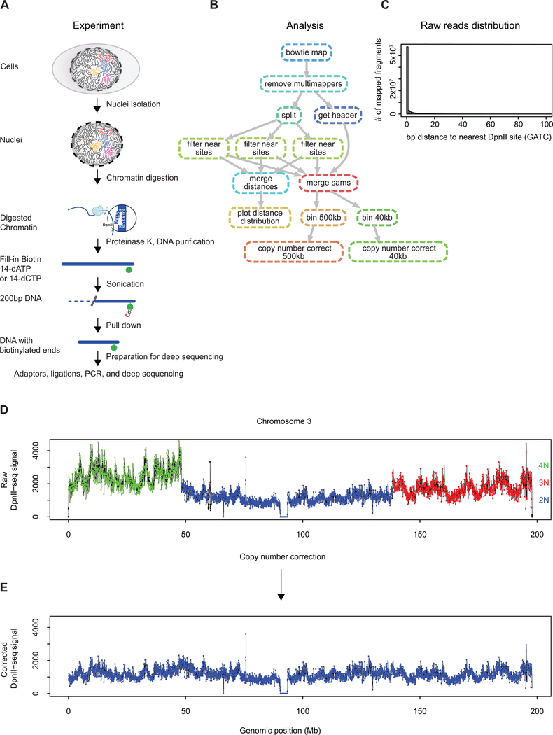
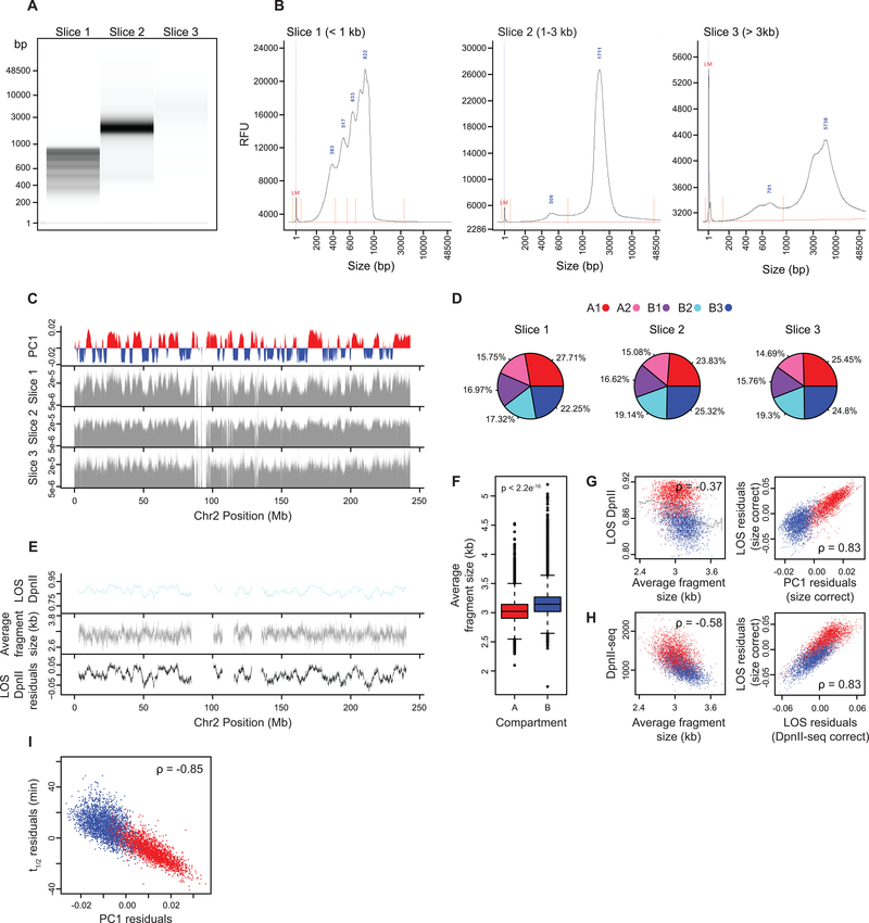
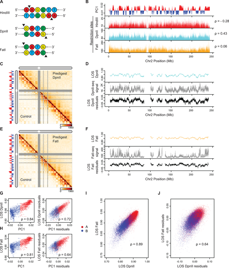
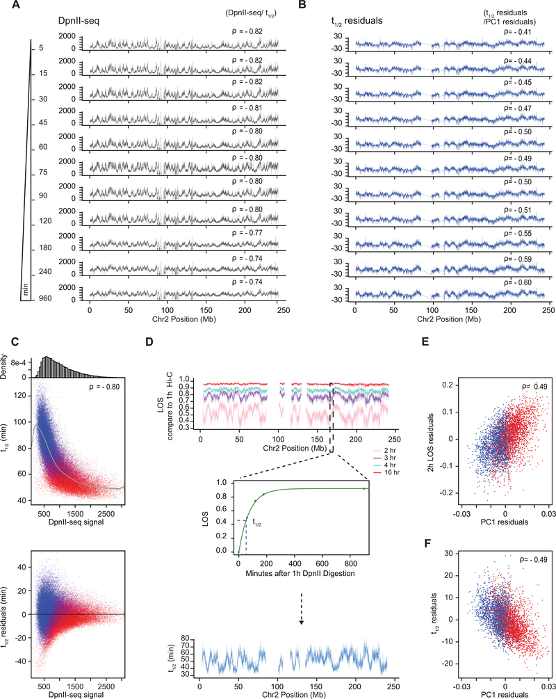
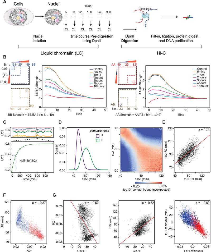
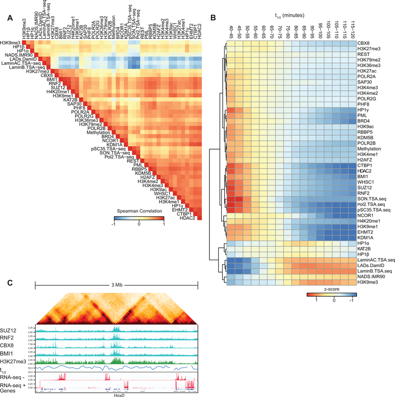
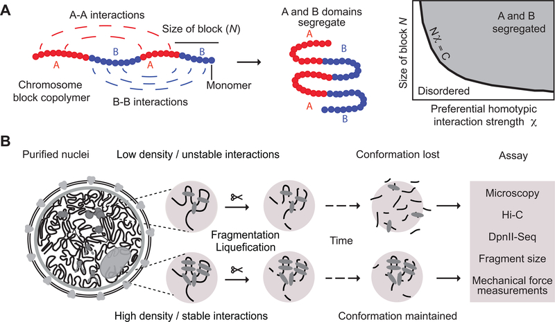
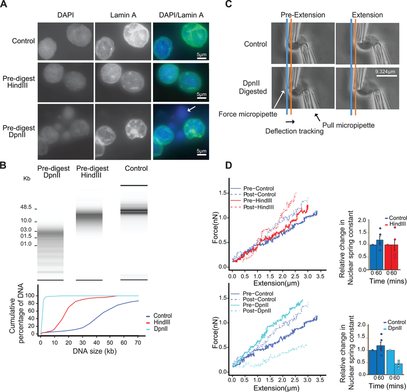
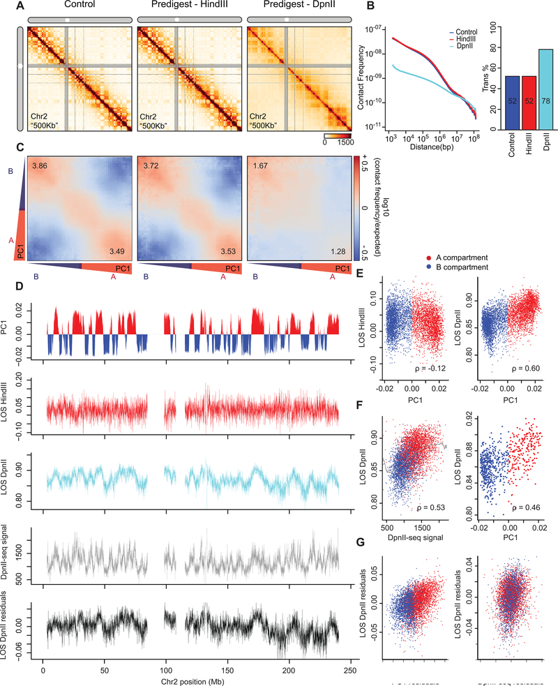
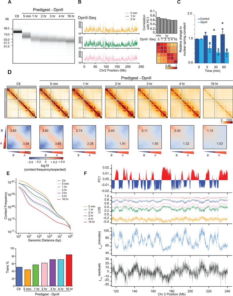
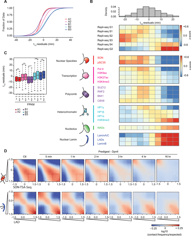
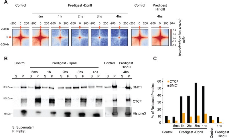
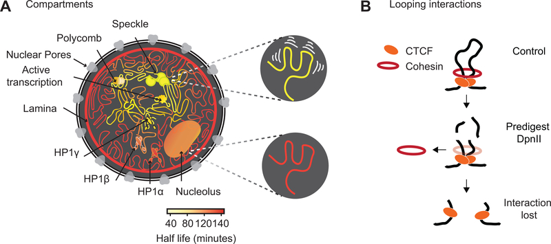
Nuclear compartmentalization of active and inactive chromatin is thought to occur through microphase separation mediated by interactions between loci of similar type. The nature and dynamics of these interactions are not known. We developed liquid chromatin Hi-C to map the stability of associations between loci. Before fixation and Hi-C, chromosomes are fragmented, which removes strong polymeric constraint, enabling detection of intrinsic locus-locus interaction stabilities. Compartmentalization is stable when fragments are larger than 10-25 kb. Fragmentation of chromatin into pieces smaller than 6 kb leads to gradual loss of genome organization. Lamin-associated domains are most stable, whereas interactions for speckle- and polycomb-associated loci are more dynamic. Cohesin-mediated loops dissolve after fragmentation. Liquid chromatin Hi-C provides a genome-wide view of chromosome interaction dynamics.


Conflict of interest statement

Competing interests statement

The authors declare no competing interests.

Figures

Extended Data Fig. 1:
Extended Data Fig. 1:. Chromosome conformation in isolated nuclei
(A) Hi-C 2.0 intra-chromosomal interaction maps for K562 cells (top) and purified nuclei (bottom). (B) 5C interaction map of 1 Mb region surrounding the beta-globin locus in K562 cells. Top: cells. Bottom: purified nuclei. CTCF-mediated interactions are preserved in purified nuclei. Red circles: positions of CTCF sites, purple square Beta-globin locus control region (LCR). (C) Representative 3C-PCR (out of two experiments) for a 44,120 kb region surrounding the beta-globin LCR on chromosome 11, detects at high resolution the known looping interactions between the LCR and the expressed gamma-globin genes (HBE1, HBG2) in K562 cells. Looping interactions are not detected in GM12878 cells that do not express these genes. Top: cells. Bottom: purified nuclei. Each data point is the average of 3 PCR reactions; error bars indicate standard error of the mean. (D) Compartmentalization saddle plots: average intra-chromosomal interaction frequencies between 100 kb bins, normalized by genomic distance. Bins are sorted by their PC1 value derived from Hi-C data obtained with K562 cells. In these plots preferential B-B interactions are in the upper left corner, and preferential A-A interactions are in the lower right corner. Numbers in the corners represent the strength of AA interactions as compared to AB interactions and BB interactions over BA interactions. Left: cells. Right: purified nuclei. (E) Spearman correlation of PC1 in cells vs PC1 in nuclei for chromosome 2 at 100kb resolution (ρ= 0.99).
Extended Data Fig. 2:
Extended Data Fig. 2:. Chromosome conformation dissolution upon chromatin fragmentation
(A) Workflow for Liquid chromatin Hi-C. (B) Illustration of loss of structure metric using a pre-digested sample and a control. (C) Hi-C interaction maps and compartmentalization saddle plots for a second replicate of control nuclei (incubated for 4 hours in restriction buffer) and nuclei pre-digested with HindIII for 4 hours. (D) Left: Spearman correlation of DpnII restriction digestion efficiency (DpnII-seq) and PC1 for chromosome 2 at 40 kb resolution. Right: Partial correlation of LOS (LOS residuals) with PC1 after controlling for restriction efficiency (DpnII-seq), for chromosome 2 at 40kb resolution. Spearman correlation is indicated. (E) compartmentalization saddle plots for the corresponding conditions. Numbers indicate strength of A-A and B-B interactions for inter-chromosomal interactions.
Extended Data Fig. 3:
Extended Data Fig. 3:. Experimental protocol and computational workflow for DpnII-seq
(A) Schematic of DpnII-seq experimental protocol for recovering DNA fragments digested by the restriction enzyme DpnII. (B) Directed graph of DpnII-seq computational pipeline (C) Histogram of distance to nearest DpnII recognition site for each recovered DpnII digested fragment. (D) Raw DpnII-seq signal displaying multiple copy number states (2N, 3N, 4N) within chromosome 3 (data binned at 40 kb). (E) Copy number corrected DpnII-seq signal displaying single copy number state (2N) across chromosome 3.
Extended Data Fig. 4:
Extended Data Fig. 4:. Average fragment size per bin and correlation with chromatin stability
(A) DNA purified from nuclei pre-digested with DpnII for 4 hours were separated into slices of three sizes and run on a Fragment Analyzer. One experiment was performed. (B) Fragment Analyzer distributions of DNA fragment sizes for the three separated slices (RFU: relative fluorescence unit, LM: lower marker, fragment sizes at distribution peaks are given in blue). (C) Top plot: Eigenvector 1 values (PC1, 40 kb resolution) across a section of chromosome 2, representing A (red) and B (blue) compartments. Bottom three plots: Normalized coverage of fragments from given slice size across a section of chromosome 2. (D) Percentages of fragments mapped to each subcompartment for given slice size. (E) Top plot: LOS along chromosome 2 at 40 kb resolution for nuclei pre-digested with DpnII. Middle plot: Average fragment size estimated for every 40kb bin after pre-digestion with DpnII (Methods). Bottom plot: LOS-residuals for nuclei pre-digested with DpnII after correction for average fragment size. (F) Boxplot of average fragment size for A compartment bins (n=35836) and B compartment bins (n=33252). Significance determined by two-sample two tailed t-test (p < 2.2e-16, t = −80.535, d.f. = 67270, 95% CI= −0.1228385,−0.1170014). Boxplot middle line is the median, the lower and upper edges of the box are the first and third quartiles, the whiskers extend to interquartile range (IQR) × 1.5 from the box. Outliers are represented as points. (G) Left plot: correlation between LOS for nuclei pre-digested with DpnII and average fragment size. Grey line indicates moving average used for residual calculation. Right plot: partial correlation between residuals of LOS for nuclei pre-digested with DpnII and residuals of PC1 after correcting for correlations between LOS and average fragment size and PC1 and average fragment size (for chromosome 2, Spearman correlation values are indicated). (H) Left plot: Correlation between DpnII-seq signal and average fragment size. Right plot: correlation between residuals of LOS after correcting for average fragment size and residuals of LOS after correcting for DpnII-seq signal (for chromosome 2, Spearman correlation values are indicated). (I) Partial correlation between residuals of t1/2 and residuals of PC1 after correcting for correlations between t1/2 and average fragment size and PC1 and average fragment size.
Extended Data Fig. 5:
Extended Data Fig. 5:. Liquid chromatin Hi-C results are reproducible using the restriction enzyme FatI
(A) Restriction sites for the selected restriction enzymes. Black triangles denote cut sites. (B) Top plot: Eigenvector 1 values (PC1, 40 kb resolution) across a section of chromosome 2, representing A (red) and B (blue) compartments. Bottom three plots: Coverage of restriction sites (40kb resolution). Spearman correlation between restriction site coverage and PC1 is given for each restriction site track. (C) Third replicate of DpnII predigest liquid chromatin Hi-C. Hi-C interaction maps of chromosome 2 binned at 500 kb. Bottom left: control nuclei in restriction buffer for 4 hours. Top right: nuclei digested for 4 hours with DpnII prior to Hi-C. Left track: Eigenvector 1 values (PC1, 40 kb resolution) across a section of chromosome 2, representing A (red) and B (blue) compartments. (D) Top plot: LOS along chromosome 2 at 40 kb resolution for nuclei pre-digested with DpnII. Middle plot: DpnII-seq signal. Bottom plot: LOS-residuals for nuclei pre-digested with DpnII after correction for DpnII-seq signal. (E) FatI predigest liquid chromatin Hi-C. Hi-C interaction maps of chromosome 2 binned at 500 kb. Bottom left: control nuclei in restriction buffer for 4 hours. Top right: nuclei digested for 4 hours with FatI prior to Hi-C. Left track: Eigenvector 1 values (PC1, 40 kb resolution) across a section of chromosome 2, representing A (red) and B (blue) compartments. (F) Top plot: LOS along chromosome 2 at 40 kb resolution for nuclei pre-digested with FatI. Middle plot: FatI-seq signal. Bottom plot: LOS-residuals for nuclei pre-digested with FatI after correction for FatI-seq signal. (G) Left plot: Correlation between LOS for nuclei pre-digested with DpnII and PC1. Right plot: partial correlation between residuals of LOS for nuclei pre-digested with DpnII and residuals of PC1 after correcting for correlations between LOS and DpnII-seq and PC1 and DpnII-seq signal (for chromosome 2, Spearman correlation values are indicated). (H) Left plot: Correlation between LOS for nuclei pre-digested with FatI and PC1. Right plot: partial correlation between residuals of LOS for nuclei pre-digested with FatI and residuals of PC1 after correcting for correlations between LOS and FatI-seq and PC1 and FatI-seq signal (for chromosome 2, Spearman correlation values are indicated). (I) Correlation between LOS for nuclei pre-digested with FatI and LOS for nuclei pre-digested with DpnII (genome wide, Spearman correlation values are indicated). (J) Correlation between residuals of LOS for nuclei pre-digested with FatI and residuals of LOS for nuclei pre-digested with DpnII after correcting for correlations between FatI LOS and FatI-seq and DpnII LOS and DpnII-seq (genome wide, Spearman correlation values are indicated).
Extended Data Fig. 6:
Extended Data Fig. 6:. Variations in Half-life and LOS are not explained by DpnII digestion kinetics
(A) DpnII-seq signals along chromosome 2 after indicated times of digestion. Spearman correlations between DpnII-seq and t1/2 at each timepoint is indicated. (B) t1/2 residuals along chromosome 2 after correcting t1/2 values by the correlation between t1/2 and DpnII-seq signals shown on the left obtained after the indicated times of digestion. Spearman correlation between t1/2 residuals and PC1 residuals are indicated. (C) Top: Genome wide scatterplot of t1/2 versus 1 hour DpnII-seq signal. Gray line: moving average. Bar plot above shows the number of loci displaying various levels of DpnII-mediated cuts. Bottom: residuals of t1/2 calculated by subtracting t1/2 from the corresponding average t1/2 (gray line in top plot) plotted vs. number of DpnII cuts. Red dots: loci in the A compartment; Blue dots: loci in the B compartment. The majority of loci have 500–1100 cuts. When comparing loci with similar number of DpnII cut we observe that loci in the A compartment have shorter t1/2 values as compared to loci in the B compartment. (D) Top: LOS along chromosome 2 at the indicated timepoints of digestion and calculated by comparison to Hi-C data obtained after 1 hour of digestion. Middle: calculation of t1/2 from LOS at different timepoints. Bottom: t1/2 along chromosome 2. This t1/2 is calculated using the Hi-C data obtained after 1 hour of pre-digestion as starting point. (E) Partial correlation between LOS and PC1 after correcting for their correlations with DpnII-seq. LOS (at 2 hours) is calculated as in panel C using the Hi-C data obtained after 1 hour of pre-digestion as starting point (F) Partial correlation between t1/2 and PC1 after correcting for their correlations with DpnII seq. t1/2 is calculated as in panel D using the Hi-C data obtained after 1 hour of pre-digestion as starting point. Spearman correlations are indicated.
Extended Data Fig. 7:
Extended Data Fig. 7:. Liquid chromatin-Hi-C protocol and quantification of loss of structure after chromatin pre-digestion
(A) Workflow for Liquid chromatin Hi-C timecourse. CL = cross-linking step. (B) Compartment strength derived from compartment saddle plots (See Methods). Left: Diagram depicting compartment strength calculation for B-B interactions. Plot to the right of diagram: B-B interaction strength as a function of bin number for all timepoints of the time course. Right: Diagram depicting compartment strength calculation for A-A interactions. Plot to the right of diagram: A-A interaction strength as a function of bin number for all time points of the time course. (C) Top: LOS signal across a 40 Mb region on chromosome 2 calculated for indicated timepoints in the digestion timecourse. Line colors as in Figure 4E. Bottom: Exponential curve fit to LOS timepoints for a single 40kb bin. t1/2 (dashed vertical blue line) representing time elapsed to reach half saturation of LOS signal. (D) Left: Density distributions of t1/2 for A and B compartments. Right: t1/2 saddle plots: average intra-chromosomal interaction frequencies between 40 kb bins, normalized by genomic distance. Bins are sorted by their t1/2 value derived from digestion timecourse. Bins with high t1/2 preferentially interact (bottom right of heatmap) and bins with low t1/2 preferentially interact (top left of heatmap). (E) Scatterplot of t1/2 vs t1/2 for two timecourse replicates (R1 and R2) on chromosome 2. Regression line (red). Spearman correlation is indicated. (F) Scatterplot of PC1 vs t1/2 for chromosome 2. A compartment (red); B compartment (blue). (G) Left: Scatterplot of percent interactions occurring in cis within a 6 Mb distance out of total genome wide interactions for each 40 kb bin in control Hi-C map (Cis %) vs PC1. Middle: Cis% vs t1/2. Right: Scatterplot of partial correlation between PC1 and t1/2 controlled by Cis %. A compartment (red); B compartment (blue). Solid red lines are regression lines. Spearman correlations are indicated.
Extended Data Fig. 8:
Extended Data Fig. 8:. Associations between sub-nuclear structures and chromatin interaction stability
(A) Spearman correlation matrix between signals for various chromatin state markers of various sub-nuclear structures, chromatin remodellers and histone modifications with row order determined by hierarchical clustering. (B) The genome was split into 16 bins, where each bin corresponds to sets of loci that share the same t1/2 interval. For each t1/2 interval the mean z-score signal enrichment for various markers of sub-nuclear structures, chromatin remodellers and histone modifications was calculated and shown as a heatmap. Row order determined by hierarchical clustering. (C) 3 Mb region surrounding HoxD locus. Top: Hi-C contact map for K562 control nuclei showing the position of the HoxD locus. Tracks: ChIP-seq tracks for polycomb subunits (cyan) and the polycomb associated histone modification H3K27me3 (green). t1/2 (blue). Minus strand and plus-strand signal of total RNA-seq (red). Refseq Genes (blue/black). The polycomb-bound domain displays shorter half-life compared to expressed genes in flanking regions.
Fig. 1:
Fig. 1:. Approach for measuring chromatin interaction stability
A: Block copolymer composed of a series of alternating A and B blocks, each composed of a number of monomers (left). The polymer can fold into spatially segregated domains of As and Bs (middle). Flory-Huggins polymer theory predicts that spatial segregation will occur when the product of the length of the blocks N (the number of monomers that make up blocks) and their effective preferential homotypic interaction strength χ (difference in the strength of homotypic interactions as compared to heterotypic (A-B) interactions) is larger than a critical value C. B: Workflow to determine the stability of chromatin interactions genome-wide. DNA: black, varying chromatin features or proteins maintaining DNA conformation: grey ovals.
Fig. 2:
Fig. 2:. Extensive fragmentation of chromatin leads to liquefied chromatin
A: Nuclear and chromatin morphology before and after chromatin fragmentation. Top row: control nuclei in restriction buffer, middle row nuclei digested for 4 hours with HindIII. Bottom row: nuclei digested for 4 hours with DpnII. Nuclei were stained with DAPI (left column), with antibodies against Lamin A (middle column). The right column shows the overlay of the DAPI and Lamin A stained images. HindIII digestion did not lead to major alteration in nuclear morphology and chromatin appearance, while DpnII digestion led to the appearance of DAPI stained droplets (arrow) exiting the nuclei. Representative images are shown, experiment repeated twice, with dozen nuclei images per experiment. B: Top: DNA purified from undigested nuclei, and nuclei pre-digested with DpnII and HindIII was run on a Fragment Analyzer. Bottom: cumulative DNA length distributions calculated from the Fragment Analyzer data. Representative data are shown for 1 out of 2 replicates. C: Micromanipulation of single nuclei. Isolated nuclei were attached to two micropipettes at opposite ends. Nuclei were extended by moving the right micropipette (Extension micropipette) and the force required was calculated from the deflection of the calibrated “force” (left) pipette. Blue and orange lines indicate the position of the force pipette before and after extension for control nuclei. After digestion of nuclei with DpnII (bottom) extension required less force as indicated by the much smaller deflection of the force pipette as compared to control nuclei (see also Supplementary Movies 1 and 2). D. Force-extension plots (left) for control nuclei before and 60 minutes after incubation in restriction buffer (pre- and post-control), for nuclei before and after digestion with DpnII, and for nuclei before and after HindIII digestion. Right panel: relative change in nuclear spring constants, calculated from the slopes of the force-extension plots shown on the left. Bars indicate standard error of the mean (n = 5 DpnII pre-digested nuclei, and n = 4 HindIII pre-digested nuclei). Bars show the average of all nuclei, dots indicate values obtained with individual nuclei.
Fig. 3:
Fig. 3:. Hi-C analysis reveals chromosome disassembly upon chromatin liquefication
(A) Hi-C interaction maps of chromosome 2 binned at 500 kb. Left: interaction map for control nuclei in restriction buffer for 4 hours. Middle: nuclei pre-digested for 4 hours with HindIII prior to Hi-C. Right: nuclei digested for 4 hours with DpnII prior to Hi-C (see Extended Data Fig. 2A). (B) Left: genome-wide interaction frequency as function of genomic distance for control nuclei (dark blue), nuclei pre-digested with HindIII (red), and nuclei pre-digested with DpnII (cyan). Right: percentage of inter-chromosomal (trans) interaction frequencies. (C) Compartmentalization saddle plots: average intra-chromosomal interaction frequencies between 40-kb bins, normalized by expected interaction frequency based on genomic distance. Bins are sorted by their PC1 value derived from Hi-C data obtained with control nuclei. In these plots preferential B-B interactions are in the upper left corner, and preferential A-A interactions are in the lower right corner. Numbers in corners represent the strength of AA interactions as compared to AB interaction and BB interactions over BA interactions. (D) Top plot: Eigenvector 1 values (PC1, 40-kb resolution) across a section of chromosome 2, representing A (red) and B (blue) compartments. Second plot: Loss of pair-wise interactions “LOS” (Methods and Extended Data Fig. 2B) along chromosome 2 at 40-kb resolution for nuclei pre-digested with HindIII. Third plot: LOS for nuclei pre-digested with DpnII. Fourth plot: DpnII-seq signal along chromosome 2 at 40-kb resolution. Bottom plot: LOS-residuals for nuclei pre-digested with DpnII after correction for DpnII signal. E) Correlation between LOS for nuclei pre-digested with HindIII (left) or DpnII (right) and PC1 (for chromosome 2, Spearman correlation values are indicated). F) Left: correlation between LOS for nuclei pre-digested with DpnII and DpnII-seq signal (for chromosome 2). Grey line indicates moving average used for residual calculation. Right: correlation between LOS for nuclei pre-digested with DpnII and PC1 for loci cut to the same extent by DpnII (1,000–1,100 DpnII-seq reads/ 40-kb bin; for chromosome 2). Spearman correlation values are indicated. G) Left: partial correlation between residuals of LOS for nuclei pre-digested with DpnII and residuals of PC1 after correcting for correlations between LOS and DpnII-seq and PC1 and DpnII-seq signal. Right: partial correlation between residuals of LOS for nuclei pre-digested with DpnII and residuals of DpnII-seq signal after correcting for correlations between LOS and PC1 and DpnII-seq signal and PC1. Spearman correlation values are indicated.
Fig. 4:
Fig. 4:. Kinetics of chromatin fragmentation and chromatin dissolution
(A) DNA purified from undigested nuclei, and nuclei pre-digested with DpnII for different time points were run on a Fragment Analyzer. Representative data are shown for 1 out of 2 replicates. (B) Left: DpnII-seq signals along chromosome 2 binned at 40-kb resolution after digestion for 5 minutes, 1 hour and 2 hours. Right: correlation between DpnII-seq signals and PC1 and between DpnII-seq signals at different time points. (C) Relative change in nuclear spring constant (nN/μm) after DpnII fragmentation at different time points. Spring constant is significantly decreased after 5 minutes and at background level by 1 hour (P = 0.002; two-tailed t-test; n = 4 or 5 nuclei except for control nuclei at t = 30 minutes where n = 2; each measured three times; error bars represent standard error of the mean). Bars show the average of all nuclei, dots indicate values obtained with individual nuclei. (D) Top row: Hi-C interaction maps of chromosome 2 binned at 500 kb. Control: nuclei in restriction buffer for 4 hours. Pre-digest DpnII: nuclei were pre-digested with DpnII for 5 minutes up to 16 hours. (Extended Data Fig. 7A). Bottom row: compartmentalization saddle plots for the corresponding conditions. Numbers indicate strength of A-A and B-B interactions for intra-chromosomal interactions. (E) Top: genome-wide interaction frequency as function of genomic distance for Hi-C data shown in panel (D). Bottom: percentage of inter-chromosomal (trans) interactions genome-wide for control nuclei and for nuclei pre-digested with DpnII for up to 16 hours. (F) Top: PC1 along a section of 120 Mb of chromosome 2. Second plot: LOS along chromosome 2 at 40-kb resolution for all time points (Extended Data Fig. 2B). Third plot: half-life (t1/2) values derived from the exponential fit of the six time-points for every 40-kb bin (Extended Data Fig. 7C). Bottom plot: residuals of t1/2 after correcting for correlations between t1/2 and DpnII-seq (DpnII-seq data for t = 1 hour).
Fig. 5:
Fig. 5:. Dissociation kinetics of chromatin interactions at different sub-nuclear structures
(A) Cumulative distributions of residuals of t1/2 (in minutes) for each of the five annotated sub-compartments. (B) Top: the genome was split into 10 bins, where each bin corresponds to sets of loci that share the same t1/2 residual interval. Middle: For each t1/2 residual interval a heatmap of mean z-score signal of Repli-Seq data in different phases of the cell cycle G1, S1–4, G2. Bottom: For each t1/2 residual interval a heatmap of mean z-score signal enrichment was quantified for various markers of sub-nuclear structures (See Methods). (C) (C) Boxplot of t1/2 residuals for bins with expressed genes (mean FPKM > 1) in sub-compartments: A1 (n = 7,045), A2 (n = 4,154), B1 (n = 1,565), B2 (n = 805), and B3 (n = 1,030) and bins with low or no expression (mean FPKM ≤1) in sub-compartments A1 (n = 3,486), A2 (n = 2,800), B1 (n = 4,726), B2 (n = 5,803), and B3 (n = 8,717). Significant difference in t1/2 residuals between expressed and non-expressed bins per subcompartment determined by two-sample two tailed t-test (A1: P = 1.04 × 10⁻⁸, t = 5.731, d.f. = 6,885.4, 95% CI = 0.57, 1.17; A2: P = 0.002, t = −3.090, d.f. = 6,072.8, 95% CI = −1.12, −0.25; B1: P = 0.493, t = −0.685, d.f. = 2,528.7, 95% CI = −0.73, 0.35; B2: P = 6.05 × 10⁻⁸, t = −5.457, d.f. = 1,051.8, 95% CI = −3.02, −1.42; B3: P = 3.29 × 10⁻¹⁰, t = −6.335, d.f. = 1,270.2, 95% CI = −2.84, −1.50). An asterisk denotes P < 0.003. Boxplot middle line is the median, the lower and upper edges of the box are the first and third quartiles, the whiskers extend to interquartile range (IQR) × 1.5 from the box. (D) Homotypic interaction saddle plots for loci ranked by their association with speckles (as detected by SON-TSA-seq, top ) and by their association with the nuclear lamina. Preferential pair-wise interactions between loci associated with the lamina can still be observed after several hours, whereas preferential pair-wise interactions between loci associated with speckles are lost more quickly.
Fig. 6:
Fig. 6:. Chromatin loop dissociation upon fragmentation
(A) Aggregated distance-normalized Hi-C interactions around 6,057 loops detected in K562 cells at 10-kb resolution, for control nuclei and nuclei digested with DpnII up to 4 hours, and for nuclei digested with HindIII for 4 hours. (B) Western blot analysis of CTCF, cohesin and histone H3 abundance in soluble (s) and chromatin-bound (p) fractions obtained from control nuclei and from nuclei pre-digested with DpnII up to 4 hours and HindIII for 4 hours. Representative data are shown for 1 out of 2 replicates. (C) Quantification of the data shown in panel B. Percentage of released protein is the ratio of protein level in the soluble fraction divided by the sum of the levels in the soluble and chromatin-bound fractions.
Fig. 7:
Fig. 7:. Illustration of chromatin interaction dynamics in the nucleus and model for cohesin loss after chromatin digestion
(A) Left: Schematic representation of varying chromatin interactions dynamics at different sub-nuclear domains. Shortest half-life reflects the least stable interactions (yellow), while longest half-life reflects the most stable interactions (dark orange). Nuclear subdomains differ greatly in their stability. Top right: Chromatin anchored at speckles is driven by the most dynamic interactions. Bottom right: Chromatin anchored at the nuclear lamina involves the most stable interactions. (B) Model for how cohesin rings stabilize CTCF-CTCF loops by encircling loop bases. Top: Cohesin ring encircles loop bases at convergent CTCF sites. Middle: Pre-digestion with DpnII cuts loop into chromatin fragments <6 kb, and the cohesin ring can slide off nearby ends. Bottom: CTCF remains bound to digested chromatin fragments but interactions between CTCF-bound sites are lost.

References

    1. Lieberman-Aiden E et al. Comprehensive mapping of long-range interactions reveals folding principles of the human genome. Science 326, 289–293 (2009). - PMC - PubMed
    1. Rao SSP et al. A 3D map of the human genome at kilobase resolution reveals principles of chromatin looping. Cell 159, 1665–1680 (2014). - PMC - PubMed
    1. Chen Y et al. Mapping 3D genome organization relative to nuclear compartments using TSA-Seq as a cytological ruler. J Cell Biol 217, 4025–4048 (2018). - PMC - PubMed
    1. Nir G et al. Walking along chromosomes with super-resolution imaging, contact maps, and integrative modeling. PLoS Genet 14, e1007872 (2018). - PMC - PubMed
    1. Wang S et al. Spatial organization of chromatin domains and compartments in single chromosomes. Science 353, 598–602 (2016). - PMC - PubMed

Publication types

LinkOut - more resources