Monitoring blood potassium concentration in hemodialysis patients by quantifying T-wave morphology dynamics

Abstract

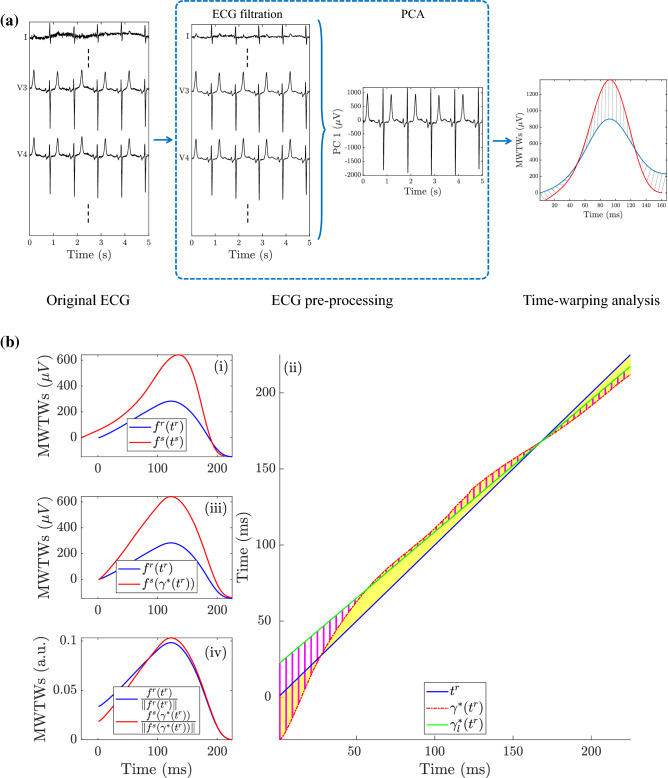
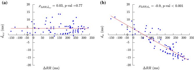
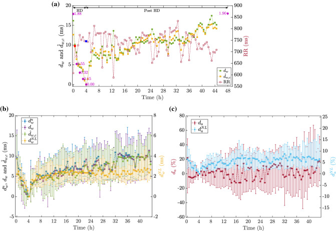
We investigated the ability of time-warping-based ECG-derived markers of T-wave morphology changes in time ([Formula: see text]) and amplitude ([Formula: see text]), as well as their non-linear components ([Formula: see text] and [Formula: see text]), and the heart rate corrected counterpart ([Formula: see text]), to monitor potassium concentration ([Formula: see text]) changes ([Formula: see text]) in end-stage renal disease (ESRD) patients undergoing hemodialysis (HD). We compared the performance of the proposed time-warping markers, together with other previously proposed [Formula: see text] markers, such as T-wave width ([Formula: see text]) and T-wave slope-to-amplitude ratio ([Formula: see text]), when computed from standard ECG leads as well as from principal component analysis (PCA)-based leads. 48-hour ECG recordings and a set of hourly-collected blood samples from 29 ESRD-HD patients were acquired. Values of [Formula: see text], [Formula: see text], [Formula: see text], [Formula: see text] and [Formula: see text] were calculated by comparing the morphology of the mean warped T-waves (MWTWs) derived at each hour along the HD with that from a reference MWTW, measured at the end of the HD. From the same MWTWs [Formula: see text] and [Formula: see text] were also extracted. Similarly, [Formula: see text] was calculated as the difference between the [Formula: see text] values at each hour and the [Formula: see text] reference level at the end of the HD session. We found that [Formula: see text] and [Formula: see text] showed higher correlation coefficients with [Formula: see text] than [Formula: see text]-Spearman's ([Formula: see text]) and Pearson's (r)-and [Formula: see text]-Spearman's ([Formula: see text])-in both SL and PCA approaches being the intra-patient median [Formula: see text] and [Formula: see text] in SL and [Formula: see text] and [Formula: see text] in PCA respectively. Our findings would point at [Formula: see text] and [Formula: see text] as the most suitable surrogate of [Formula: see text], suggesting that they could be potentially useful for non-invasive monitoring of ESRD-HD patients in hospital, as well as in ambulatory settings. Therefore, the tracking of T-wave morphology variations by means of time-warping analysis could improve continuous and remote [Formula: see text] monitoring of ESRD-HD patients and flagging risk of [Formula: see text]-related cardiovascular events.

Figure 1

Diagram of the study protocol: $h_0$ to $h_5$ are the time points (in minutes) for blood sample extraction. $h_4$ is taken at the end of the HD (minute 215-th or 245-th, depending on the HD duration).

Figure 2

Analysis stages performed in this study. In panel (a) is the flow chart showing the ECG processing steps for T-wave time-warping markers extraction. The analysis starts with the original ECG, followed by a filtering step before spatial PCA analysis, to conclude with markers computation. Panel (b) shows an example of the linear and nonlinear time-warping markers for the same patient as in Fig. 5a. In particular, subpanel (i) shows both the reference (blue) and the i-th MWTW (red) while subpanel (ii) shows the warping function (red dotted line) that optimally relates the reference and studied MWTWs. Subpanel (iii) shows the MWTWs after warping and subpanel (iv) are the normalized reference and warped MWTWs.

Figure 3

Scatterplot showing the values of both $d_w$ panel (a) and ${\widehat{d}}_{w,c}$ panel (b) with respect to $\mathrm{\Delta }RR$ for a given patient in PCA approach. Spearman’s correlation coefficients ($\rho$) and p-values for both $d_w$ and ${\widehat{d}}_{w,c}$ are shown on top of each panel, while the least-square fitting regression lines are plotted in red.

Figure 4

Boxplots showing the distribution of $\mathrm{\Delta }[K^{+}]$ (blue) and all the described PCA-based time-warping biomarkers ($d_w^u$, $d_a$, $d_w^{\mathrm{NL}}$, $d_a^{\mathrm{NL}}$, $d_w$, and ${\widehat{d}}_{w,c}$) (red), computed at different time points from the beginning, $h_0$, to the end, $h_4$, of the HD session ($h_0$ to $h_4$ in Fig. 1). $\mathrm{\Delta }[K^{+}]$ was computed as in (23). + denotes outliers.

Figure 5

PCA-based time-warping markers and RR interval time trends. An example for a given patient undergoing 4h-long HD therapy, is depicted in panel (a) with the evolution of $d_w$ (filled green squares), ${\widehat{d}}_{w,c}$ (filled orange squares), both referring to the left vertical scale, and the average RR intervals (unfilled dark red squares, referring to the right vertical scale). $\mathrm{\Delta }[K^{+}]$ relative variations with respect to the concentration at HD end (purple diamonds) are expressed in mmol/L. Time is expressed in hours from the beginning of the treatment onward. Each square denotes the mean RR interval in a 2-min wide segment used to compute the warping parameters, while the highlighted blue square corresponds to the reference segment at the end of HD. The filled red square denotes the time-point from which the studied MWTW in Fig. 2b was selected. Note that for this patient, the Holter recording did not reach the planned 48h. Panel (b) shows the median and IQR for each observing i-th segment, computed by using the values from all the available patients for $d_w^u$, $d_w$ and ${\widehat{d}}_{w,c}$ and $d_w^{\mathrm{NL}}$ (this latter refers to the right axis, while the others to the left). Time trends (expressed as median and IQR) for $d_a$ and $d_a^{\mathrm{NL}}$, referring to the left and right axes respectively are in panel (c). Panels (b) and (c) give an overview of the time evolution for these biomarkers along the ECG acquisition from the HD beginning onward. Only the first 44 h were depicted being that the average ECG duration in our database.

References

1. KDIGO Definition and classification of CKD. Kidney Int. Suppl. 2013;3:16–92. doi: 10.1038/kisup.2012.64. - DOI - PMC - PubMed
1. Grassmann A, Gioberge S, Moeller S, Brown G. ESRD patients in 2004: Global overview of patient numbers, treatment modalities and associated trends. Nephrol. Dial. Transplant. 2005;20:2587–2593. doi: 10.1093/ndt/gfi159. - DOI - PubMed
1. Makar MS, Pun PH. Sudden cardiac death among hemodialysis patients. Am. J. Kidney Dis. 2017;69:684–695. doi: 10.1053/j.ajkd.2016.12.006. - DOI - PMC - PubMed
1. Secemsky EA, et al. High prevalence of cardiac autonomic dysfunction and T-wave alternans in dialysis patients. Heart Rhythm. 2010;8:592–598. doi: 10.1016/j.hrthm.2010.11.041. - DOI - PubMed
1. Pitt B, Rossignol P. The association between serum potassium and mortality in patients with hypertension: A wake-up call. Eur. Heart J. 2016;38:113–115. doi: 10.1093/eurheartj/ehw209. - DOI - PubMed
Publication types