Music-selective neural populations arise without musical training

Abstract

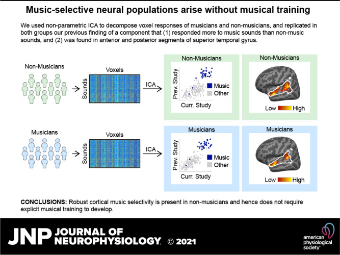
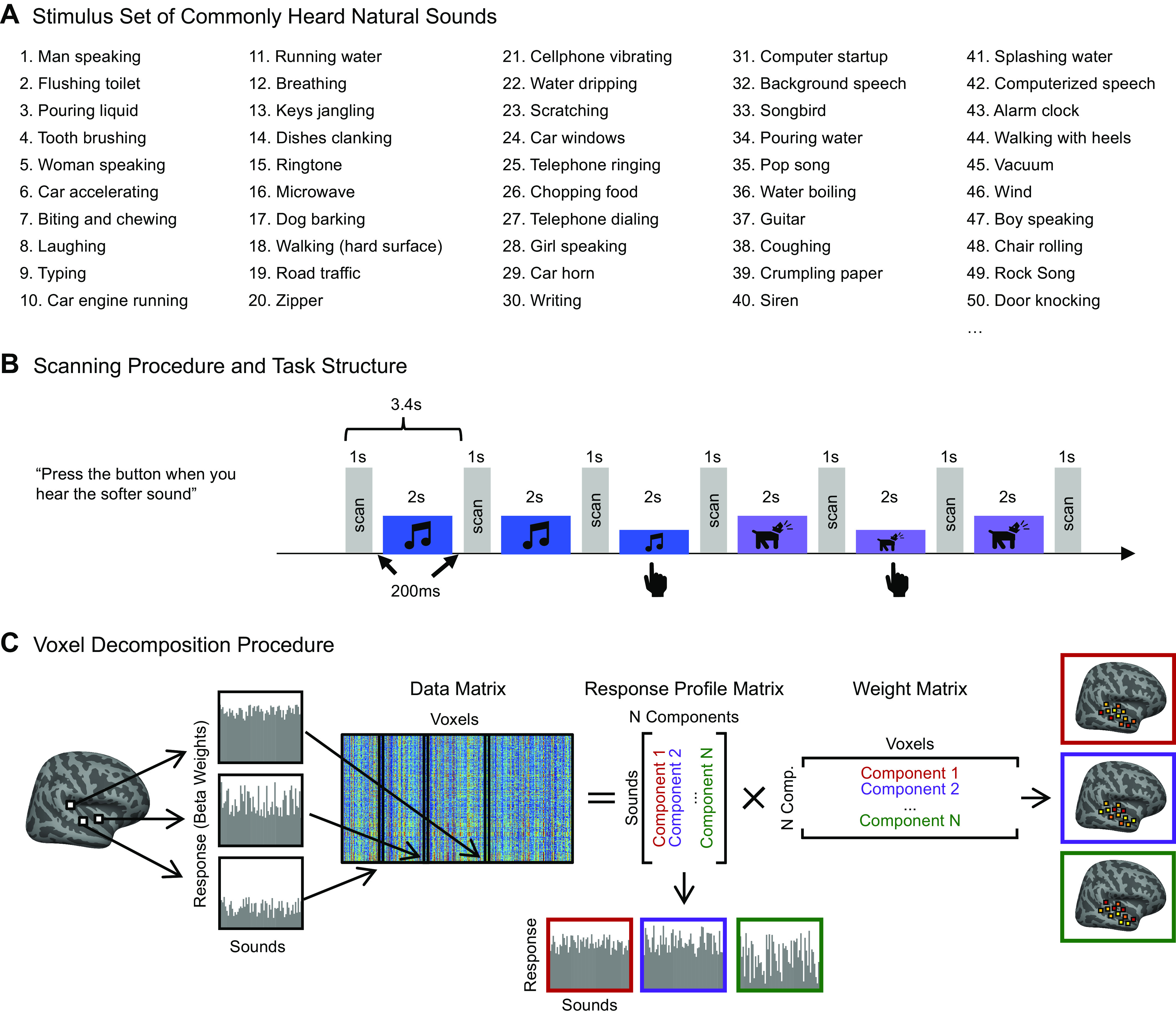
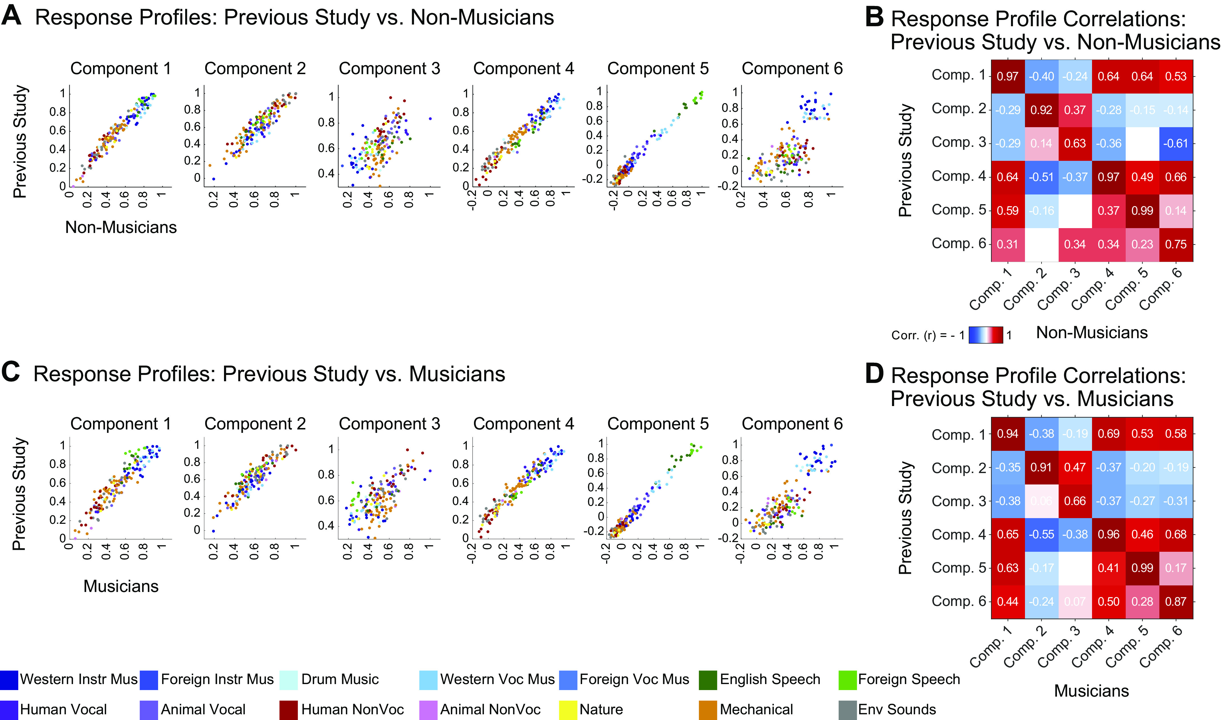
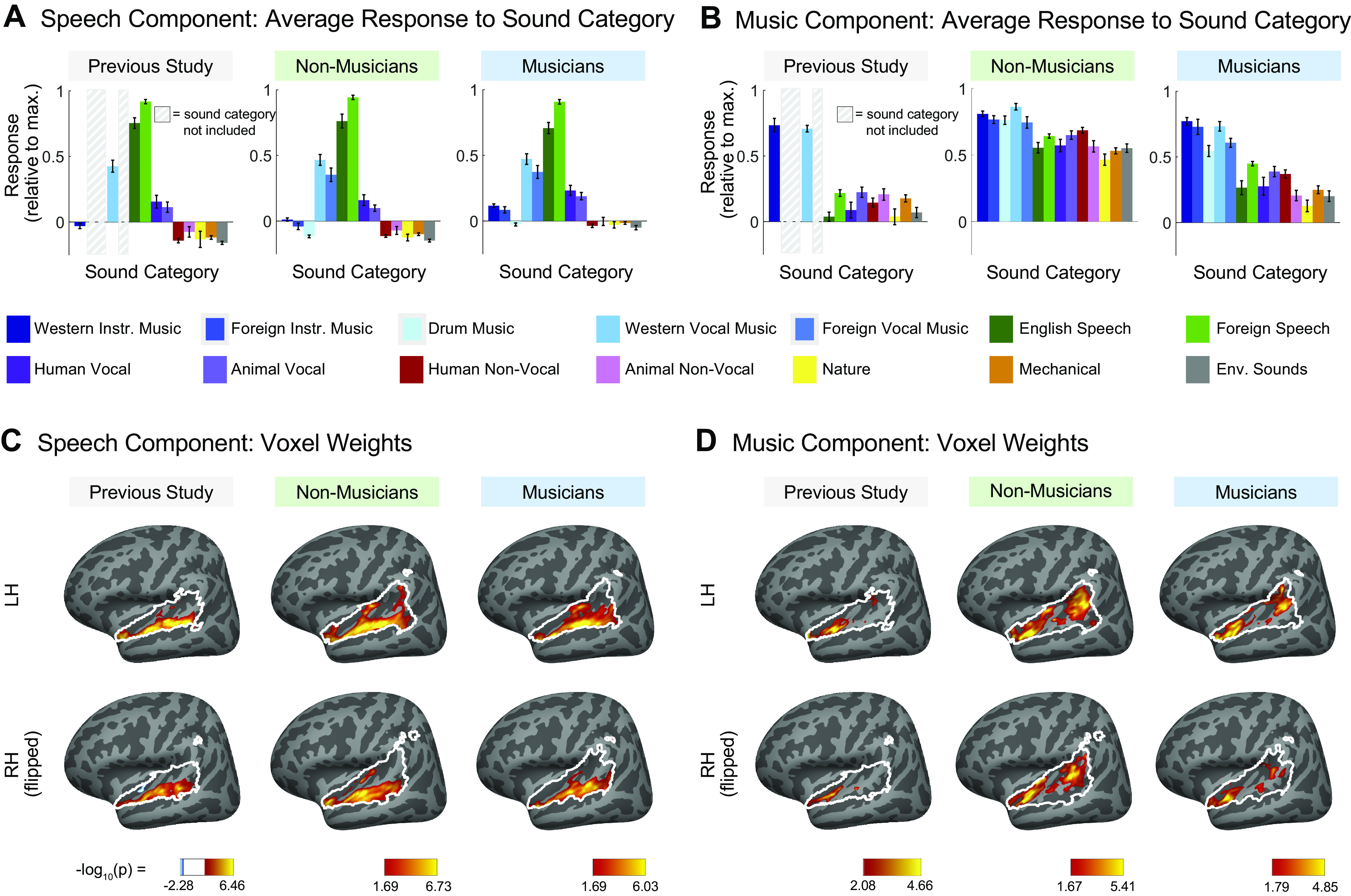
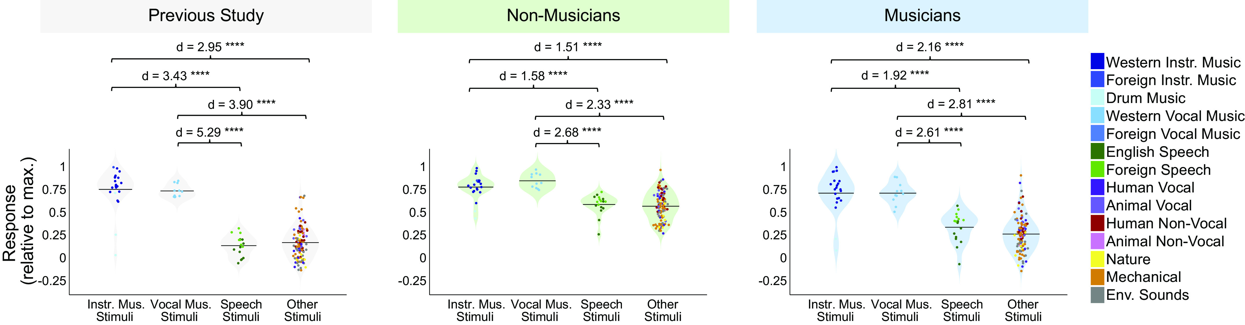
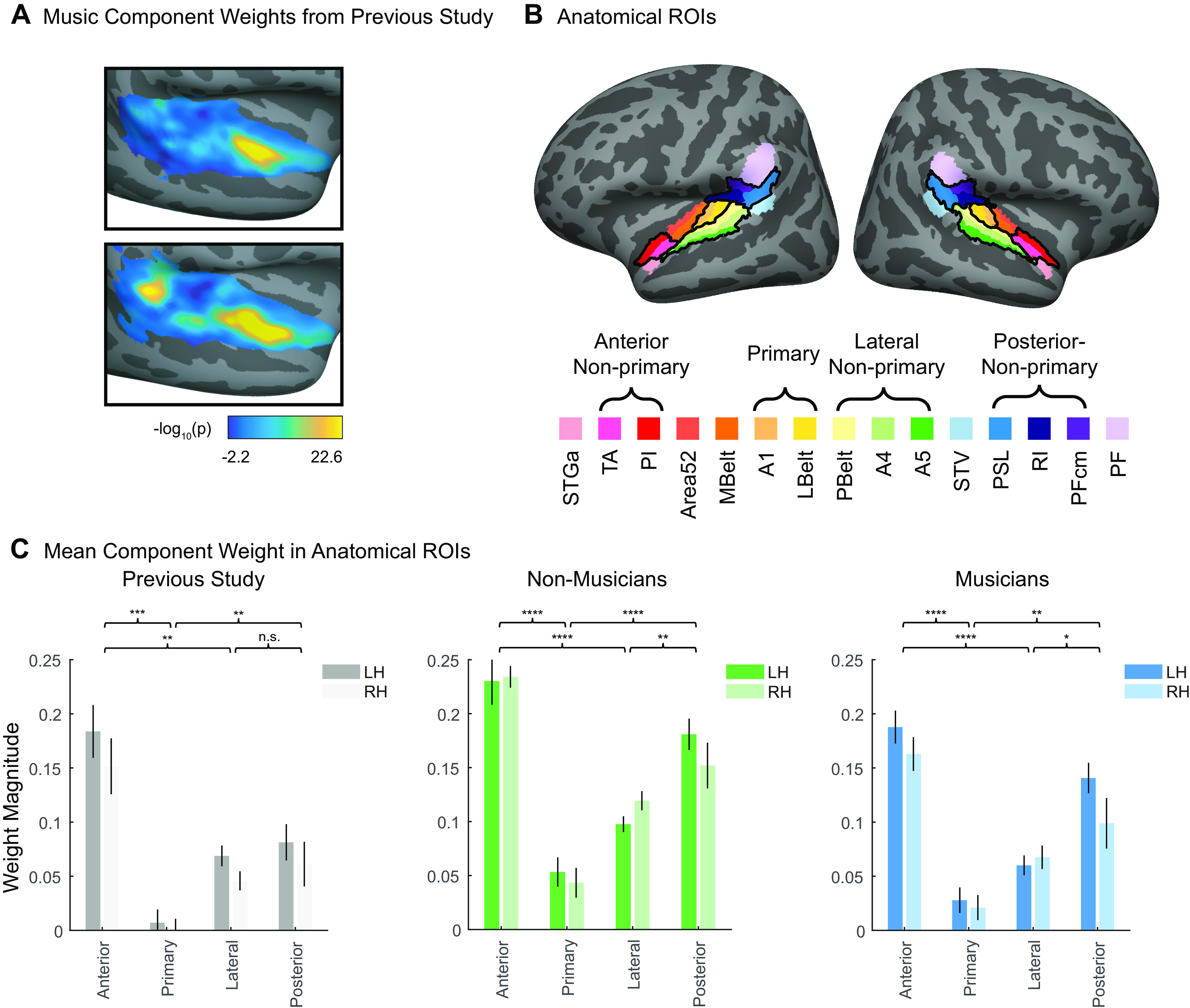
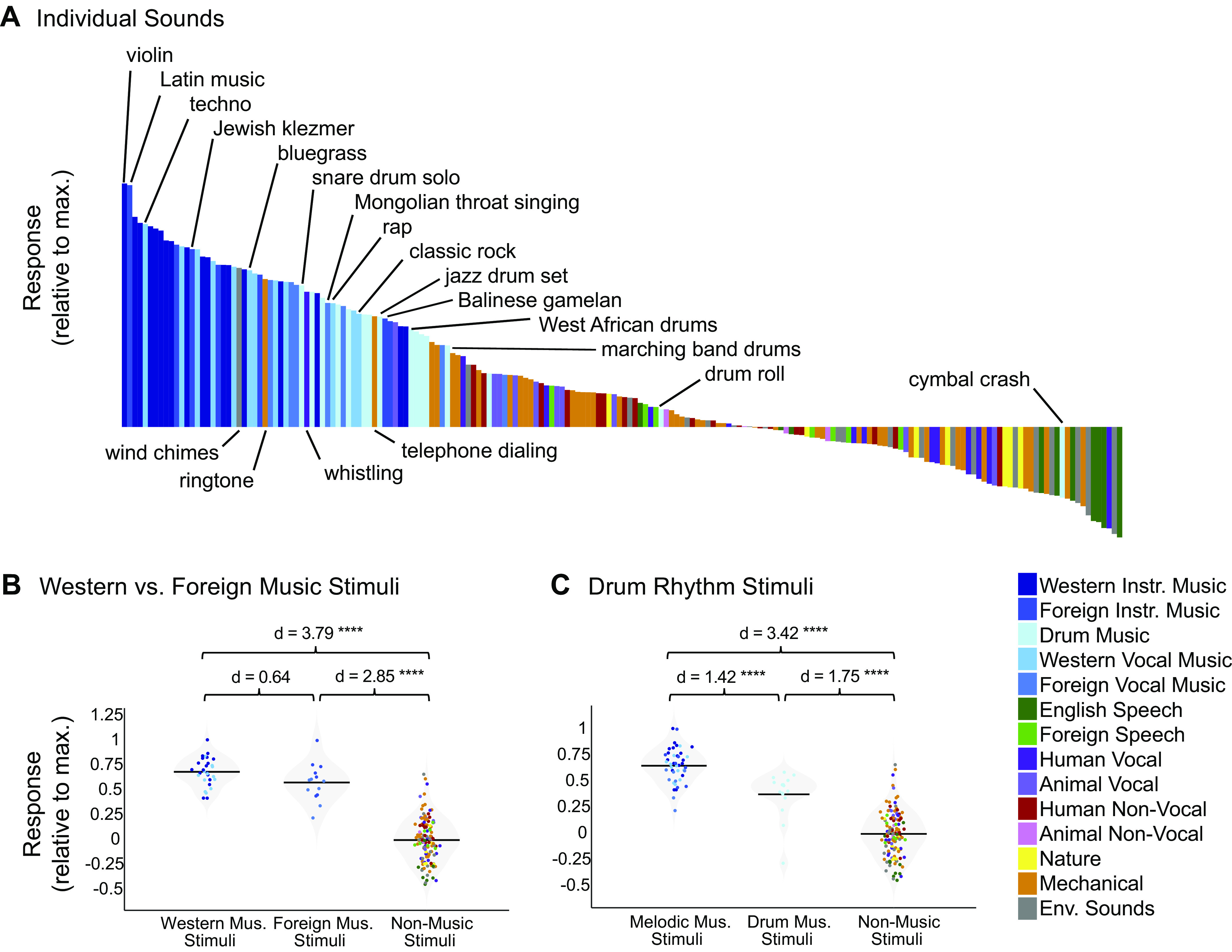
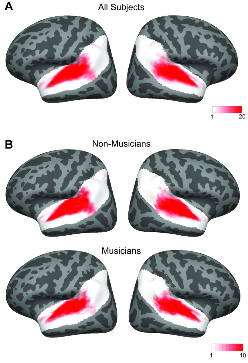
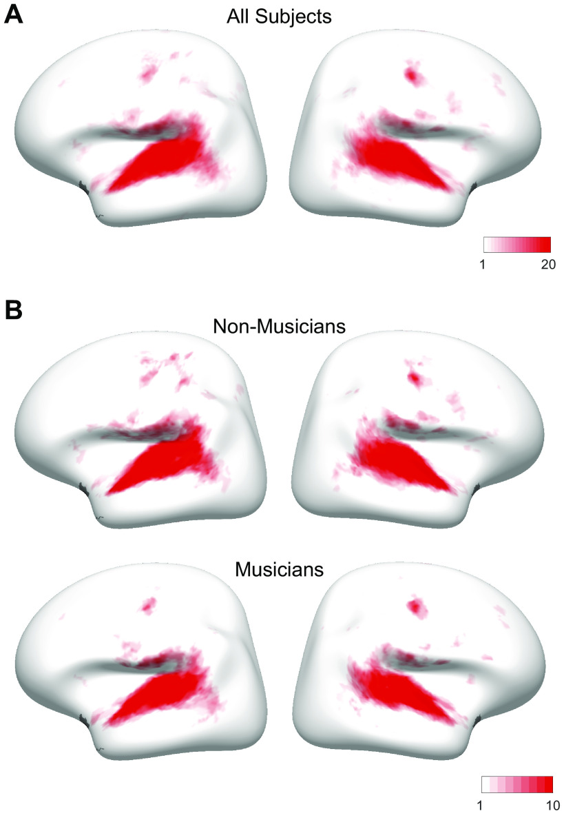
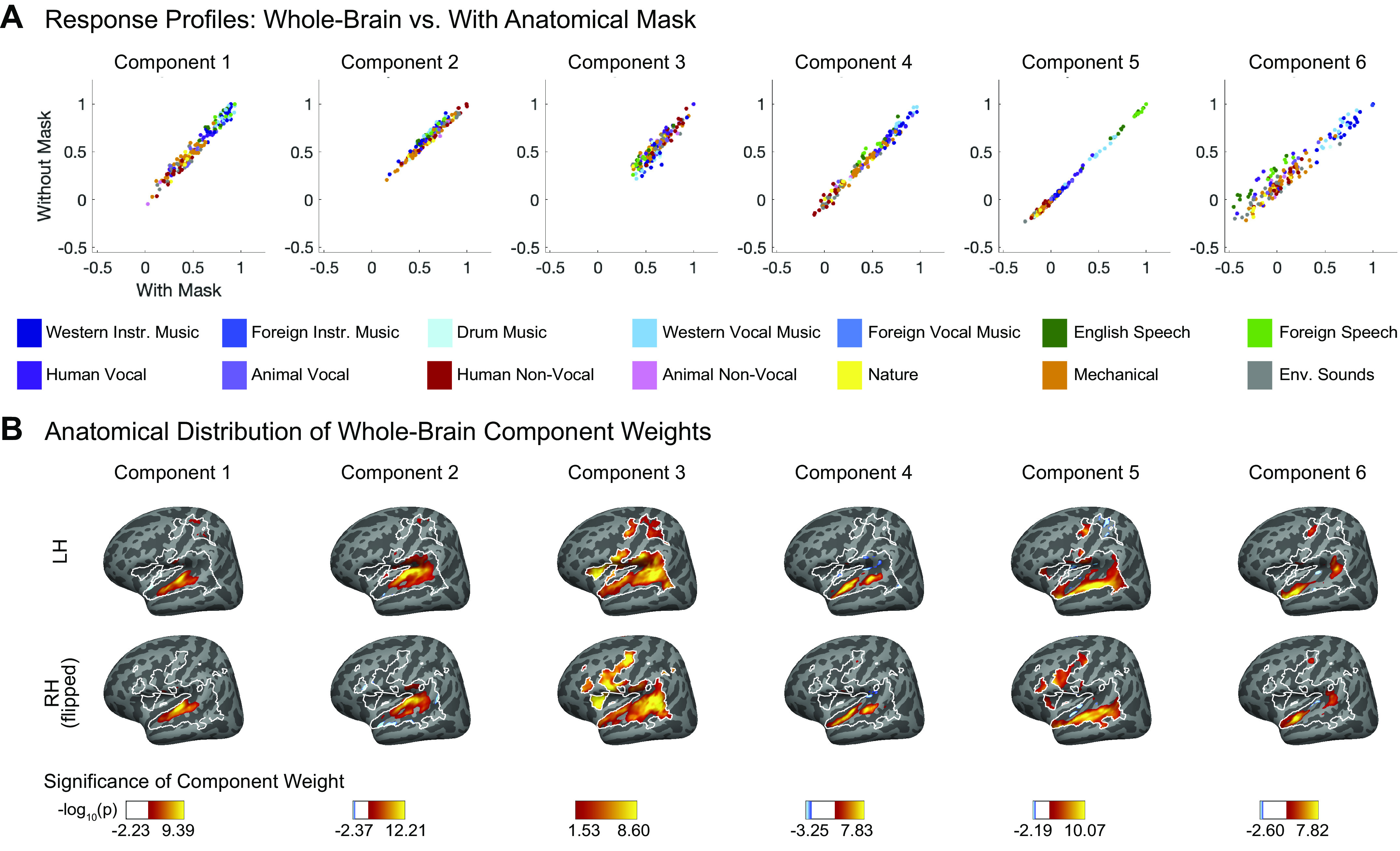
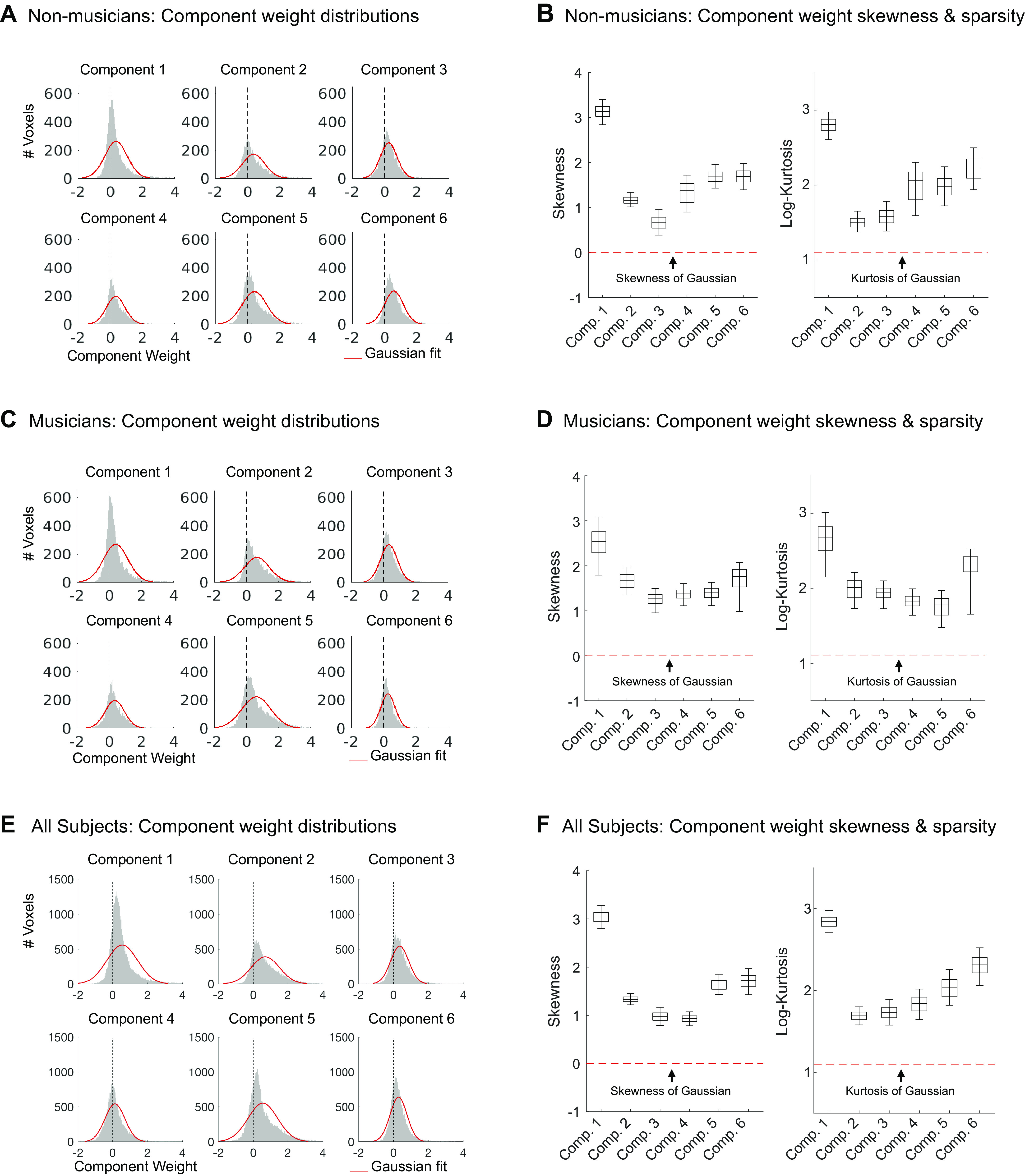
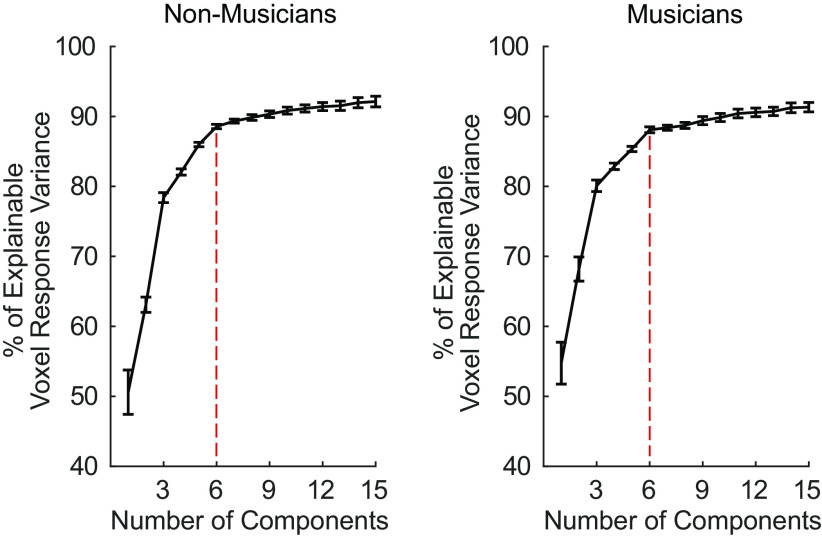
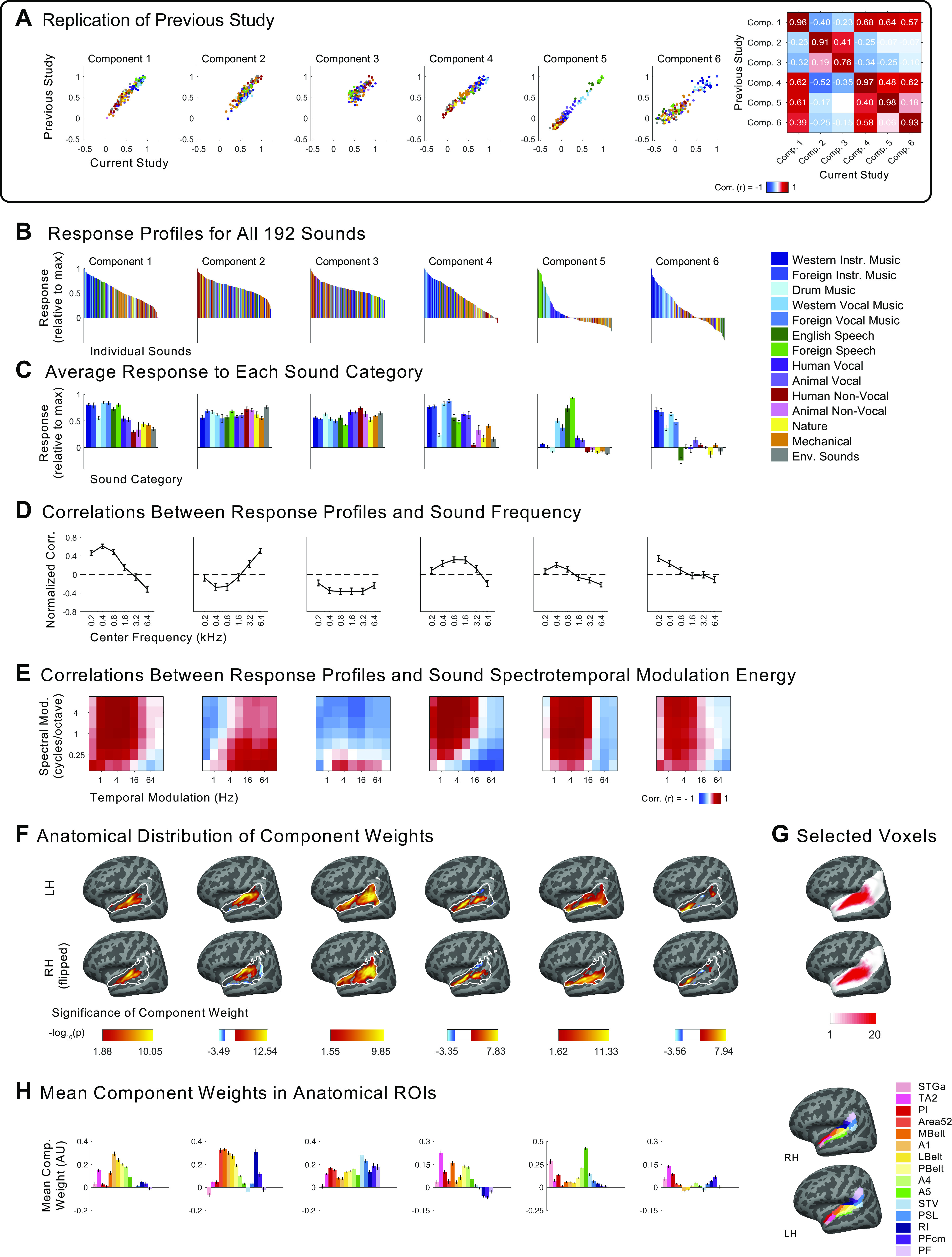
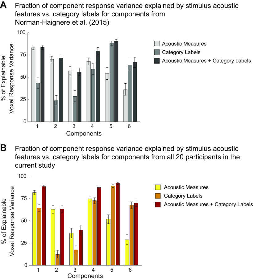
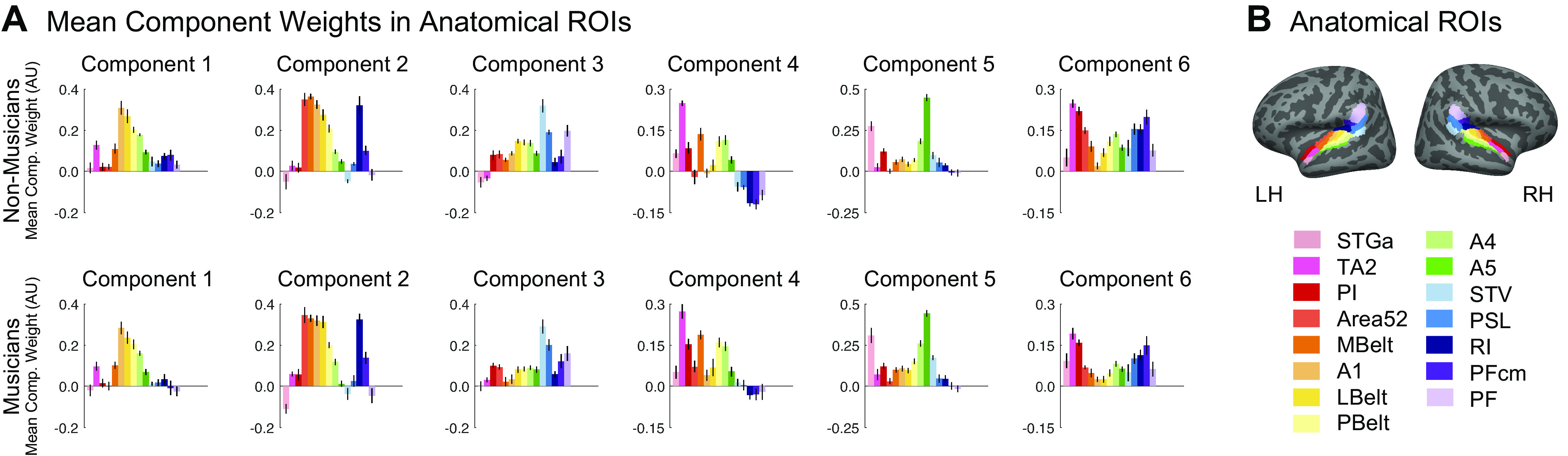
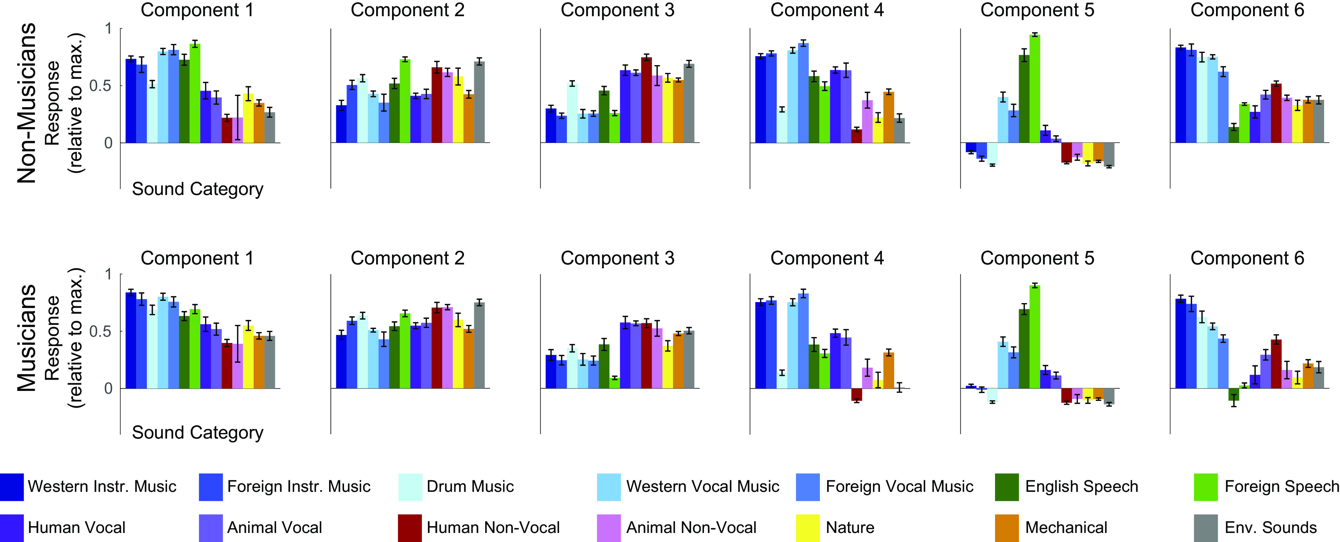
Recent work has shown that human auditory cortex contains neural populations anterior and posterior to primary auditory cortex that respond selectively to music. However, it is unknown how this selectivity for music arises. To test whether musical training is necessary, we measured fMRI responses to 192 natural sounds in 10 people with almost no musical training. When voxel responses were decomposed into underlying components, this group exhibited a music-selective component that was very similar in response profile and anatomical distribution to that previously seen in individuals with moderate musical training. We also found that musical genres that were less familiar to our participants (e.g., Balinese gamelan) produced strong responses within the music component, as did drum clips with rhythm but little melody, suggesting that these neural populations are broadly responsive to music as a whole. Our findings demonstrate that the signature properties of neural music selectivity do not require musical training to develop, showing that the music-selective neural populations are a fundamental and widespread property of the human brain.NEW & NOTEWORTHY We show that music-selective neural populations are clearly present in people without musical training, demonstrating that they are a fundamental and widespread property of the human brain. Additionally, we show music-selective neural populations respond strongly to music from unfamiliar genres as well as music with rhythm but little pitch information, suggesting that they are broadly responsive to music as a whole.

Keywords: auditory cortex; decomposition; expertise; fMRI; music.

Graphical abstract

Figure 1.

Experimental design and voxel decomposition method. A: fifty examples from the original set of 165 natural sounds used in Ref. and in the current study, ordered by how often participants reported hearing them in daily life. An additional 27 music stimuli were added to this set of 165 for the current experiment. B: scanning paradigm and task structure. Each 2-s sound stimulus was repeated three times consecutively, with one repetition (the second or third) being 12 dB quieter. Subjects were instructed to press a button when they detected this quieter sound. A sparse scanning sequence was used, in which one fMRI volume was acquired in the silent period between stimuli. C: diagram depicting the voxel decomposition method, reproduced from Ref. . The average response of each voxel to the 192 sounds is represented as a vector, and the response vector for every voxel from all 20 subjects is concatenated into a matrix (192 sounds × 26,792 voxels). This matrix is then factorized into a response profile matrix (192 sounds × N components) and a voxel weight matrix (N components × 26,792 voxels).

Figure 2.

Replication of components from Ref. . A: scatterplots showing the correspondence between the component response profiles from the previous study (n = 10, y-axis) and those inferred from nonmusicians (n = 10, x-axis). The 165 sounds common to both studies are colored according to their semantic category, as determined by raters on Amazon Mechanical Turk. Note that the axes differ slightly between groups to make it possible to clearly compare the pattern of responses across sounds independent of the overall response magnitude. B: correlation matrix comparing component response profiles from the previous study (y-axis) and those inferred from nonmusicians (n = 10, x-axis). C and D: same as A and B but for musicians. Comp., component.

Figure 3.

Comparison of speech-selective and music-selective components for participants from previous study (n = 10), nonmusicians (n = 10), and musicians (n = 10). A and B: component response profiles averaged by sound category (as determined by raters on Amazon Mechanical Turk). A: the speech-selective component responds highly to speech and music with vocals, and minimally to all other sound categories. Shown separately for the previous study (left), nonmusicians (middle), and musicians (right). Note that the previous study contained only a subset of the stimuli (165 sounds) used in the current study (192 sounds) so some conditions were not included and are thus replaced by a gray rectangle in the plots and surrounded by a gray rectangle in the legend. B: the music-selective component (right) responds highly to both instrumental and vocal music, and less strongly to other sound categories. Note that “Western Vocal Music” stimuli were sung in English. We note that the mean response profile magnitude differs between groups, but that selectivity as measured by separability of music and nonmusic is not affected by this difference (see text for explanation). For both A and B, error bars plot one standard error of the mean across sounds from a category, computed using bootstrapping (10,000 samples). C: spatial distribution of speech-selective component voxel weights in both hemispheres. D: spatial distribution of music-selective component voxel weights. Color denotes the statistical significance of the weights, computed using a random effects analysis across subjects comparing weights against 0; P values are logarithmically transformed (−log₁₀[P]). The white outline indicates the voxels that were both sound-responsive (sound vs. silence, P < 0.001 uncorrected) and split-half reliable (r > 0.3) at the group level (see materials and methods for details). The color scale represents voxels that are significant at FDR q = 0.05, with this threshold computed for each component separately. Voxels that do not survive FDR correction are not colored, and these values appear as white on the color bar. The right hemisphere (bottom rows) is flipped to make it easier to visually compare weight distributions across hemispheres. Note that the secondary posterior cluster of music component weights is not as prominent in this visualization of the data from Ref. due to the thresholding procedure used here; we found in additional analyses that a posterior cluster emerged if a more lenient threshold is used. FDR, false discovery rate; LH, left hemisphere; RH, right hemisphere.

Figure 4.

Separability of sound categories in music-selective components of nonmusicians and musicians. Distributions of 1) instrumental music stimuli, 2) vocal music stimuli, 3) speech stimuli, and 4) other stimuli within the music component response profiles from our previous study (n = 10; left, gray shading), as well as those inferred from nonmusicians (n = 10; center, green shading) and musicians (n = 10; right, blue shading). The mean for each stimulus category is indicated by the horizontal black line. The separability between pairs of stimulus categories (as measured using Cohen’s d) is shown above each plot. The 165 individual sounds are colored according to their semantic category. Stimuli consisted of instrumental music (n = 22), vocal music (n = 11), speech (n = 17), and other (n = 115). See Table 2 for results of pairwise comparisons indicated by brackets; ****Significant at P < 0.0001, two-tailed.

Figure 5.

Quantification of bilateral anterior/posterior concentration of voxel weights for the music-selective components inferred in nonmusicians and musicians separately. A: music component voxel weights, reproduced from Ref. . See materials and methods for details concerning the analysis and plotting conventions from our previous paper. B: fifteen standardized anatomical parcels were selected from Ref. , chosen to fully encompass the superior temporal plane and superior temporal gyrus (STG). To come up with a small set of ROIs to use to evaluate the music component weights in our current study, we superimposed these anatomical parcels onto the weights of the music component from our previously published study (7), and then defined ROIs by selecting sets of the anatomically defined parcels that correspond to regions of high (anterior nonprimary, posterior nonprimary) vs. low (primary, lateral nonprimary) music component weights. The anatomical parcels that comprise these four ROIs are indicated by the brackets and outlined in black on the cortical surface. C: mean music component weight across all voxels in each of the four anatomical ROIs, separately for each hemisphere, and separately for our previous study (n = 10; left, gray shading), nonmusicians (n = 10; center, green shading), and musicians (n = 10; right, blue shading). A repeated-measures ROI × hemisphere ANOVA was conducted for each group separately. Error bars plot one standard error of the mean across participants. Brackets represent pairwise comparisons that were conducted between ROIs with expected high vs. low component weights, averaged over hemisphere. See Table 3 for full results of pairwise comparisons, and Fig. A9 for component weights from all 15 anatomical parcels. *Significant at P < 0.05, two-tailed; **Significant at P < 0.01, two-tailed; ***Significant at P < 0.001, two-tailed; ****Significant at P < 0.0001, two-tailed. Note that because of our prior hypotheses and the significance of the omnibus F test, we did not correct for multiple comparisons. LH, left hemisphere; RH, right hemisphere; ROI, region of interest.

Figure 6.

A: close-up of the response profile (192 sounds) for the music component inferred from all participants (n = 20), with example stimuli labeled. Note that there are a few “nonmusic” stimuli (categorized as such by Amazon Mechanical Turk raters) with high component rankings, but that these are all arguably musical in nature (e.g., wind chimes, ringtone). Conversely, “music” stimuli with low component rankings (e.g., “drumroll” and “cymbal crash”) do not contain salient melody or rhythm, despite being classified as “music” by human listeners. B: distributions of Western music stimuli (n = 30), non-Western music stimuli (n = 14), and nonmusic stimuli (n = 132) within the music component response profile inferred from all 20 participants, with the mean for each stimulus group indicated by the horizontal black line. The separability between categories of stimuli (as measured using Cohen’s d) is shown above the plot. Note that drum stimuli were left out of this analysis. C: distributions of melodic music stimuli (n = 44), drum rhythm stimuli (n = 16), and nonmusic stimuli (n = 132) within the music component response profile inferred from all 20 participants, with the mean for each stimulus group indicated by the horizontal black line. The separability between categories of stimuli (as measured using Cohen’s d) is shown above the plot, and significance was evaluated using a nonparametric test permuting stimulus labels 10,000 times. ****Significant at P < 0.0001, two-tailed. Sounds are colored according to their semantic category.

Figure A1.

Musicians (n = 10) outperform nonmusicians (n = 10) on psychoacoustic tasks. A: participants’ pure tone frequency discrimination thresholds were measured using a 1-up 3-down adaptive two-alternative forced choice (2AFC) task, in which participants indicated which of two pairs of tones were different in frequency. Note that lower thresholds correspond to better performance. B: sensorimotor synchronization abilities were measured by instructing participants to tap along with an isochronous beat at various tempos and comparing the standard deviation of the difference between participants’ response onsets and the actual stimulus onsets. C: melody discrimination was measured using a 2AFC task, in which participants heard two five-note melodies (with the second one transposed up by a tritone) and were asked to judge whether the two melodies were the same or different. D: we measured participants’ ability to determine whether a melody conforms to the rules of Western music theory by creating 16-note melodies using a probabilistic generative model of Western tonal melodies (112) and instructing participants to determine whether or not the melody contained an out-of-key (“sour”) note. Colored dots represent individual participants, and the median for each participant group is indicated by the horizontal black line. Mus., musicians; Non-Mus., nonmusicians. *Significant at P < 0.01 one-tailed, **Significant at P < 0.001 one-tailed.

Figure A2.

Subject overlap maps showing which voxels were selected in individual subjects to serve as input to the voxel decomposition algorithm. The white area shows the anatomical constraint regions from which voxels were selected. A: overlap map for all 20 subjects. B: overlap maps for nonmusicians (n = 10) and musicians (n = 10) separately, illustrating that the anatomical location of the selected voxels was largely similar across groups.

Figure A3.

Subject overlap maps showing which voxels pass the selection criteria as described in Fig. A2, but without any anatomical mask applied before selecting voxels.

Figure A4.

Similarity between components with anatomical mask vs. whole-brain. A: scatter plots showing the components inferred from all 20 participants, using the voxel decomposition algorithm both with and without the anatomical mask shown in Fig. A2. Individual sounds are colored according to their semantic category. B: spatial distribution of whole brain component voxel weights, computed using a random effects analysis of participants’ individual component weights. Weights are compared against 0; P values are logarithmically transformed (−log₁₀[P]). The white outline indicates the voxels that were both sound-responsive (sound vs. silence, P < 0.001 uncorrected) and split-half reliable (r > 0.3) at the group level. The color scale represents voxels that are significant at FDR q = 0.05, with this threshold being computed for each component separately. Voxels that do not survive FDR correction are not colored, and these values appear as white on the color bar. The right hemisphere (bottom row) is flipped to make it easier to visually compare weight distributions across hemispheres. FDR, false discovery rate.

Figure A5.

A: histograms showing the weight distributions for each component inferred from nonmusicians (n = 10), along with their Gaussian fits (red). B: skewness and log-kurtosis (a measure of sparsity) for each component inferred from nonmusicians (n = 10), illustrating that the inferred components are skewed and sparse compared with a Gaussian (red dotted lines). Box-and-whisker plots show central 50% (boxes) and central 95% (whiskers) of the distribution for each statistic (via bootstrapping across subjects). For both the weight distribution histograms and analyses of non-Gaussianity, we used independent data to infer components (runs 1–24) and to measure the statistical properties of the component weights (runs 25–48). C and D: same as A and B, but for the components inferred from musicians (n = 10). E and F: same as A and B, but for the components inferred from all 20 participants. Comp, component.

Figure A6.

The proportion of voxel response variance explained by different numbers of components, for both nonmusicians (n = 10, left) and musicians (n = 10, right). The figure plots the median variance explained across voxels (noise corrected by split-half reliability using the Spearman correction for attenuation; 121), calculated separately for each subject and then averaged across the 10 subjects in each group. Error bars plot one standard error of the mean across subjects. For both groups, six components were sufficient to explain over 88% of the noise-corrected variance.

Figure A7.

Independent components inferred from voxel decomposition of auditory cortex of all 20 participants (as compared with the components in Figs. 2–5, which were inferred from musicians and nonmusicians separately). Additional plots are included here to show the extent of the replication of the results of Ref. . A: scatterplots showing the correspondence between the components from our previous study (n = 10; y-axis) and those from the current study (n = 20; x-axis). Only the 165 sounds that were common between the two studies are plotted. Sounds are colored according to their semantic category, as determined by raters on Amazon Mechanical Turk. B: response profiles of components inferred from all participants (n = 20), showing the full distribution of all 192 sounds. Sounds are colored according to their category. Note that “Western Vocal Music” stimuli were sung in English. C: the same response profiles as above, but showing the average response to each sound category. Error bars plot one standard error of the mean across sounds from a category, computed using bootstrapping (10,000 samples). D: correlation of component response profiles with stimulus energy in different frequency bands. E: correlation of component response profiles with spectrotemporal modulation energy in the cochleograms for each sound. F: spatial distribution of component voxel weights, computed using a random effects analysis of participants’ individual component weights. Weights are compared against 0; P values are logarithmically transformed (−log₁₀[P]). The white outline indicates the 2,249 voxels that were both sound-responsive (sound vs. silence, P < 0.001 uncorrected) and split-half reliable (r > 0.3) at the group level. The color scale represents voxels that are significant at FDR q = 0.05, with this threshold being computed for each component separately. Voxels that do not survive FDR correction are not colored, and these values appear as white on the color bar. The right hemisphere (bottom row) is flipped to make it easier to visually compare weight distributions across hemispheres. G: subject overlap maps showing which voxels were selected in individual subjects to serve as input to the voxel decomposition algorithm (same as Fig. A2A). To be selected, a voxel must display a significant (P < 0.001, uncorrected) response to sound (pooling over all sounds compared to silence) and produce a reliable response pattern to the stimuli across scanning sessions (see equations in materials and methods section). The white area shows the anatomical constraint regions from which voxels were selected. H: mean component voxel weights within standardized anatomical parcels from Ref. , chosen to fully encompass the superior temporal plane and superior temporal gyrus (STG). Error bars plot one standard error of the mean across participants. LH, left hemisphere; RH, right hemisphere; ROI, region of interest.

Figure A8.

Total amount of component response variation explained by 1) all acoustic measures (frequency content and spectrotemporal modulation energy), 2) all category labels (as assigned by Amazon Mechanical Turk workers), and 3) the combination of acoustic measures and category labels. A: results for components from our previous study (n = 10; 7). For components 1–4, category labels explained little additional variance beyond that explained by acoustic features. For components 5 (speech-selective) and 6 (music-selective), category labels explained most of the response variance, and acoustic features accounted for little additional variance. B: same as A but for the components inferred from all 20 participants in the current study.

Figure A9.

A: mean component weight in a set of 15 anatomical parcels from Glasser et al. (64), plotted separately for nonmusicians (n = 10; top) and musicians (n = 10; bottom). Error bars plot one standard error of the mean across participants. B: selected anatomical parcels from Glasser et al. (64), chosen to fully encompass the superior temporal plane and superior temporal gyrus (STG). LH, left hemisphere; RH, right hemisphere; ROI, region of interest.

Figure A10.

Response profiles discovered using the probabilistic parametric method, separately for nonmusicians (n = 10; top) and musicians (n = 10; bottom). These components were very highly correlated with those inferred using the nonparametric ICA-based voxel decomposition method presented in the main text, with the main difference between the two methods being the mean response profile magnitude (i.e., the “offset” from baseline). Because this mean response varies depending on the details of the analysis used to infer the components, while the components themselves remain highly similar, we chose to quantify selectivity using a measure (Cohen’s d) that does not take the baseline into account but rather quantifies the separation between stimulus categories within the response profile. ICA, independent components analysis.

References

1. Mehr SA, Singh M, Knox D, Ketter DM, Pickens-jones D, Atwood S, Lucas C, Egner A, Jacoby N, Hopkins EJ, Howard M, Donnell TJO, Pinker S, Krasnow MM, Glowacki L. Universality and diversity in human song. Science 366: eaax0868, 2019. doi:10.1126/science.aax0868. - DOI - PMC - PubMed
1. Trehub SE. The developmental origins of musicality. Nat Neurosci 6: 669–673, 2003. doi:10.1038/nn1084. - DOI - PubMed
1. Fedorenko E, McDermott JH, Norman-Haignere SV, Kanwisher NG. Sensitivity to musical structure in the human brain. J Neurophysiol 108: 3289–3300, 2012. doi:10.1152/jn.00209.2012. - DOI - PMC - PubMed
1. LaCroix AN, Diaz AF, Rogalsky C. The relationship between the neural computations for speech and music perception is context-dependent: an activation likelihood estimate study. Front Psychol 6: 1–19, 2015. doi:10.3389/fpsyg.2015.01138. - DOI - PMC - PubMed
1. Leaver AM, Rauschecker JP. Cortical representation of natural complex sounds: effects of acoustic features and auditory object category. J Neurosci 30: 7604–7612, 2010. doi:10.1523/JNEUROSCI.0296-10.2010. - DOI - PMC - PubMed
LinkOut - more resources