Where did they not go? Considerations for generating pseudo-absences for telemetry-based habitat models

Abstract

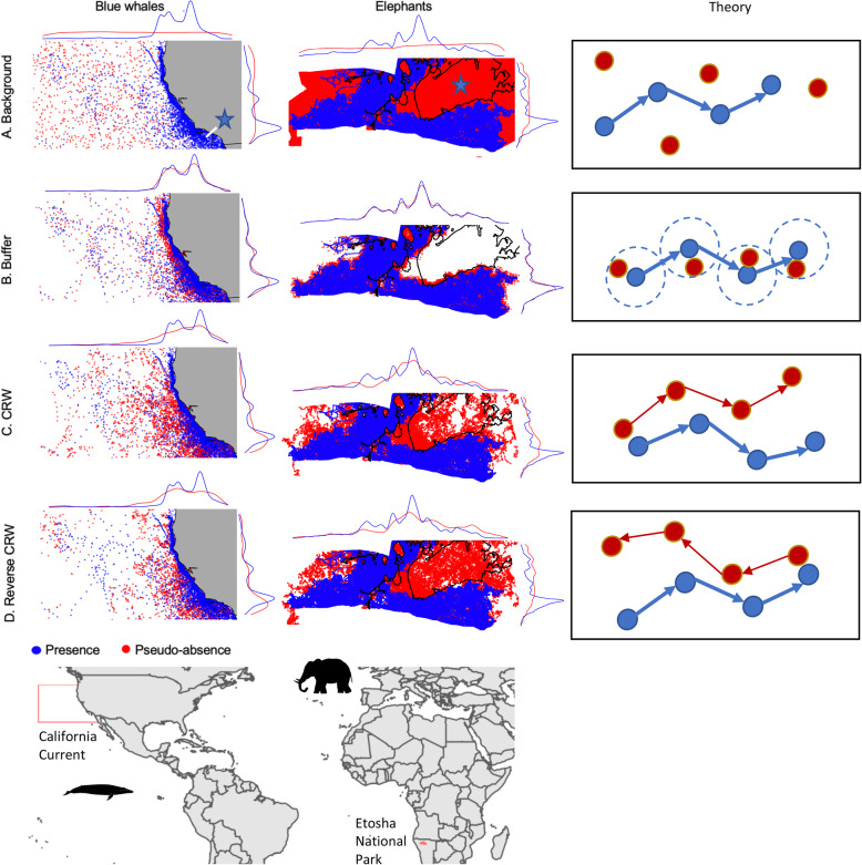
Background: Habitat suitability models give insight into the ecological drivers of species distributions and are increasingly common in management and conservation planning. Telemetry data can be used in habitat models to describe where animals were present, however this requires the use of presence-only modeling approaches or the generation of 'pseudo-absences' to simulate locations where animals did not go. To highlight considerations for generating pseudo-absences for telemetry-based habitat models, we explored how different methods of pseudo-absence generation affect model performance across species' movement strategies, model types, and environments.

Methods: We built habitat models for marine and terrestrial case studies, Northeast Pacific blue whales (Balaenoptera musculus) and African elephants (Loxodonta africana). We tested four pseudo-absence generation methods commonly used in telemetry-based habitat models: (1) background sampling; (2) sampling within a buffer zone around presence locations; (3) correlated random walks beginning at the tag release location; (4) reverse correlated random walks beginning at the last tag location. Habitat models were built using generalised linear mixed models, generalised additive mixed models, and boosted regression trees.

Results: We found that the separation in environmental niche space between presences and pseudo-absences was the single most important driver of model explanatory power and predictive skill. This result was consistent across marine and terrestrial habitats, two species with vastly different movement syndromes, and three different model types. The best-performing pseudo-absence method depended on which created the greatest environmental separation: background sampling for blue whales and reverse correlated random walks for elephants. However, despite the fact that models with greater environmental separation performed better according to traditional predictive skill metrics, they did not always produce biologically realistic spatial predictions relative to known distributions.

Conclusions: Habitat model performance may be positively biased in cases where pseudo-absences are sampled from environments that are dissimilar to presences. This emphasizes the need to carefully consider spatial extent of the sampling domain and environmental heterogeneity of pseudo-absence samples when developing habitat models, and highlights the importance of scrutinizing spatial predictions to ensure that habitat models are biologically realistic and fit for modeling objectives.

Fig. 1

Presence data (blue points) and pseudo-absence data (red points) for the four pseudo-absence generation techniques a background, b buffer, c Correlated Random Walks (CRWs), d reverse CRW for blue whales (left), elephants (middle), and in theory (right). White represents areas unvisited by tagged individuals or simulated pseudo-absences. Density by latitude (top of panel) and longitude (right side of panel) highlights the difference in pseudo-absence sampling approach (red) from observed habitat using tracking data (blue). The Southern California Bight (top left) and salt pans (middle left) are indicated with blue stars. Study domains of the California Current, U.S. and Etosha National Park, Namibia are shown in the bottom two panels. In the right-most panels, the theory behind calculation of pseudo-absences for each approach is shown with blue being actual positions and red being simulated positions

Fig. 2

Degree of environmental separation for key predictor variables between presences (black line) and each pseudo-absence generation technique (colors) for blue whales (a-d), and elephants (e-g). Grey shading represents overlap across all techniques

Fig. 3

Relationship between model predictive skill (AUC; Area Under the Receiver Operating Characteristic Curve) and environmental separation between presences and pseudo-absences (Bhattacharyya’s coefficient) for blue whales (upper) and elephants (lower). Bhattacharyya’s coefficient was calculated for key environmental covariates (symbols). Sub-panels for each model type (BRT, GAMM, GLMM) are shown, with colors indicating pseudo-absence generation technique. The lines represent linear regression between the AUC value and the Bhattacharyya’s coefficient independent of pseudo-absence type and variable

Fig. 4

Effect of pseudo-absence generation type for BRT (a-d, four panels on left), GAMM (e-h), and GLMM models (i-l) and model type using background sampling (a, e, i - top three panels), buffer sampling (b, f, j), CRW sampling (c, g, k), and reverse CRW sampling (d, h, l) on blue whale model predictions for a given day, August 1st, 2006. Yellow indicates high habitat suitability while blue is low habitat suitability. GLMMs and GAMMs have white pixels where there were missing predictor variables (e.g. due to cloud cover) for the day. The blue star in panel A is pointing to the Southern California Bight

Fig. 5

Effect of pseudo-absence generation type for elephants for BRT (a-d, four panels on left), GAMM (e-h), and GLMM models (i-l) and model type using background sampling (a, e, i, top three panels), buffer sampling (b, f, j), CRW sampling (c, g, k), and reverse CRW sampling (d, h, l) Yellow indicates high habitat suitability while blue is low habitat suitability

References

-
- Aarts G, MacKenzie M, McConnell B, Fedak M, Matthiopoulos J. Estimating space-use and habitat preference from wildlife telemetry data. Ecography. 2008;31:140–160.
- Abrahms B, Welch H, Brodie S, Jacox MG, Becker EA, Bograd SJ, Irvine LM, Palacios DM, Mate BR, Hazen EL. Dynamic ensemble models to predict distributions and anthropogenic risk exposure for highly mobile species. Divers Distrib. 2019;25(8):1182–1193.
- Allouche O, Tsoar A, Kadmon R. Assessing the accuracy of species distribution models: prevalence, kappa and the true skill statistic (TSS) J Appl Ecol. 2006;43:1223–1232.
LinkOut - more resources
Full Text Sources
Other Literature Sources