Epidemiological model for the inhomogeneous spatial spreading of COVID-19 and other diseases

Abstract

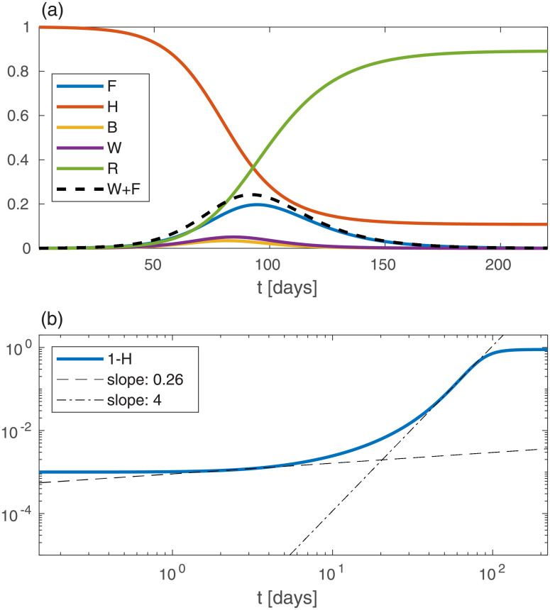
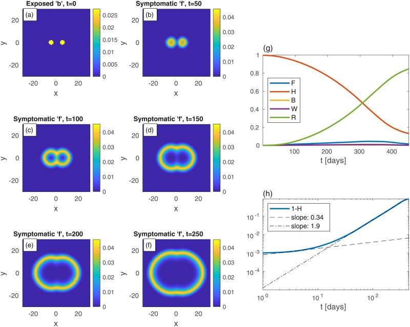
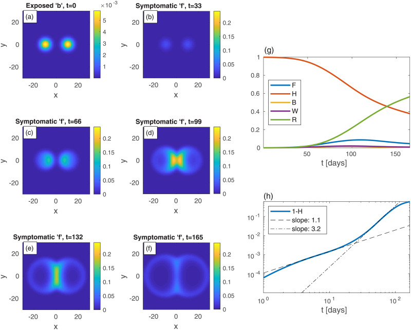
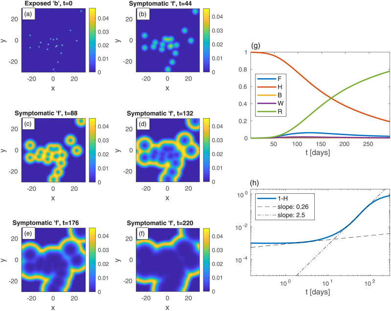
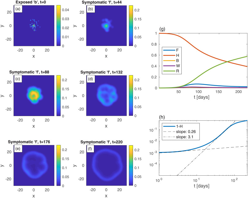
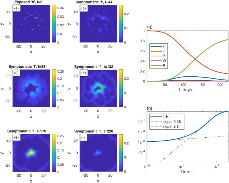
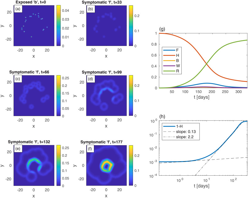
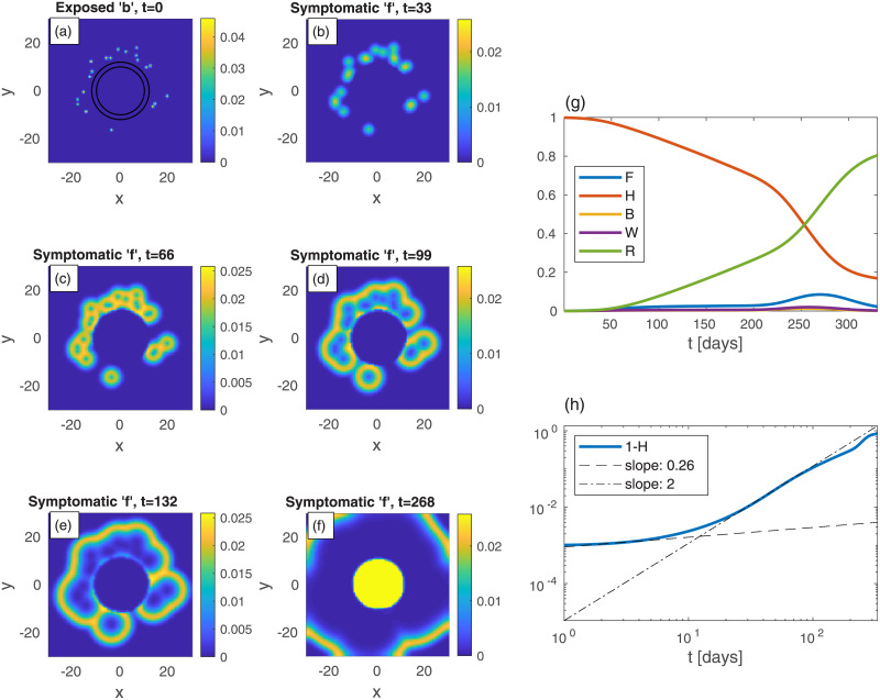
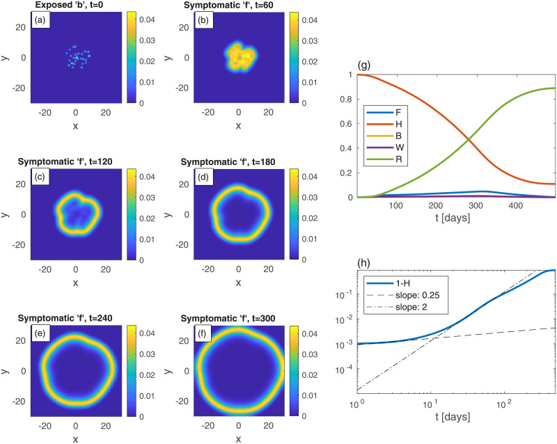
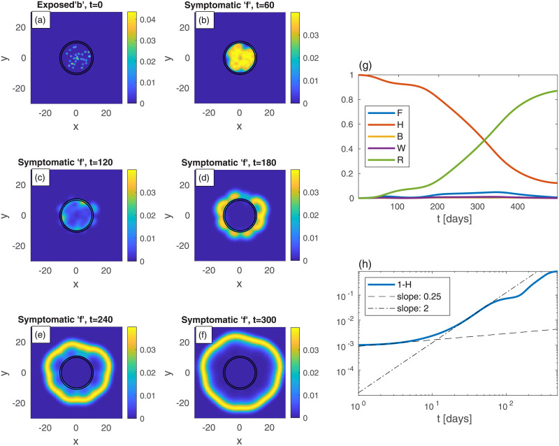
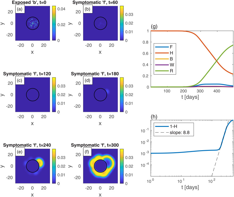
We suggest a novel mathematical framework for the in-homogeneous spatial spreading of an infectious disease in human population, with particular attention to COVID-19. Common epidemiological models, e.g., the well-known susceptible-exposed-infectious-recovered (SEIR) model, implicitly assume uniform (random) encounters between the infectious and susceptible sub-populations, resulting in homogeneous spatial distributions. However, in human population, especially under different levels of mobility restrictions, this assumption is likely to fail. Splitting the geographic region under study into areal nodes, and assuming infection kinetics within nodes and between nearest-neighbor nodes, we arrive into a continuous, "reaction-diffusion", spatial model. To account for COVID-19, the model includes five different sub-populations, in which the infectious sub-population is split into pre-symptomatic and symptomatic. Our model accounts for the spreading evolution of infectious population domains from initial epicenters, leading to different regimes of sub-exponential (e.g., power-law) growth. Importantly, we also account for the variable geographic density of the population, that can strongly enhance or suppress infection spreading. For instance, we show how weakly infected regions surrounding a densely populated area can cause rapid migration of the infection towards the populated area. Predicted infection "heat-maps" show remarkable similarity to publicly available heat-maps, e.g., from South Carolina. We further demonstrate how localized lockdown/quarantine conditions can slow down the spreading of disease from epicenters. Application of our model in different countries can provide a useful predictive tool for the authorities, in particular, for planning strong lockdown measures in localized areas-such as those underway in a few countries.

Fig 1. Solution of the epidemic model for the case of spatially uniform population densities n, b, h, w, f, and r, against the time t (in units of days).

(a) Curves depicting the global sub-population fractions (capital letters), amounting here to simple multiplication of the local densities by the area. The initial conditions are B = 10⁻³ and W = F = R = 0. (b) A log-log plot of the cumulative infected population, 1 − H, vs time (in days). The dashed and dash-dotted lines are fits at t = 2 and t = 55, respectively. In this and in all other figures D_k = 0.03, k = 0.15 days⁻¹, γ₀ = 1/2 days⁻¹, γ₁ = 1/3 days⁻¹, γ₂ = 1/13.6 days⁻¹.

Fig 2. Time evolution of an epidemic starting from two infection centers (in this and in all other figures, t is the time in days, and x and y are the spatial Cartesian coordinates).

(a) Initial conditions of b. B—the global value of b—is the same as in Fig 1. n is uniform and all other populations are initially zero: w = f = r = 0. Panels (b)-(f) depict the spreading pattern of the symptomatic population ‘f’ as time progresses. The two circular domains grow and merge into one oval-like domain. Panel (g) shows the global sub-populations F, H, B, W, and R vs time t (in days). Panel (h) shows the cumulative fraction of infected population 1 − H vs time t in (in days) on a log-log scale. Compare to the cases of uniform (Fig 1). Dashed and dash-dotted curves in panel are linear fits at t = 3 and t = 150, respectively.

Fig 3

Time evolution of a epidemic starting from two infection centers near a heavily populated region, see (a) (top-left panel); t is the time given in days, and x and y are the spatial Cartesian coordinates. n is non-uniform and given by $n\left(\mathbf{r}\right)=10a{e}^{-r^2/{\ell }^2}+a$, with ℓ = 10 and a taken such that the spatial average of n is 0.2; see Fig SI-1 in S1 File for illustration. The global value of b is the same as in previous figures, B = 10⁻³, and all other populations are initially zero everywhere: w = f = r = 0. Panels (b)-(f) show the spread of the symptomatic population f as time progresses. The symptomatic population quickly spreads into the denser region in the center and its density there increases dramatically. The global sub-population fractions, and the cumulative fraction of infected population 1 − H, are shown in panels (g) and (h), respectively.

Fig 4. Time evolution of an epidemic with randomly scattered infection centers; t is the time given in days, and x and y are the spatial Cartesian coordinates.

(a) At t = 0 (top-left panel), there are small infection centers of the exposed sub-population b scattered randomly in space. The global value of b (B) is the same as in Fig 1, i.e. B = 10⁻³. n is uniform and all other populations are set initially to zero: w = f = r = 0. Panels (b)-(f) show the spread of the symptomatic population f as time progresses. Panel (g) shows the global sub-populations F, H, B, W, and R vs time t (in days), and panel (h) shows the cumulative fraction of infected population 1 − H vs time in on a log-log scale. Dashed and dash-dot curves are linear fits at t = 2 and t = 73, respectively. In Fig SI-2 in S1 File we plot heat-maps of 1 − h—the corresponding cumulative infections.

Fig 5

Time evolution of an epidemic starting from multiple infection centers inside a heavily populated region (“city”, panel (a)); t is the time given in days, and x and y are the spatial Cartesian coordinates. The population density of the city n is nonuniform and given by $n\left(\mathbf{x}\right)=10a{e}^{-x^2/{\ell }^2}+a$, with x = (x,y), ℓ = 10, and a taken such that the spatial average of n is 0.2; see Fig SI-1 in S1 File for illustration. The integrated initial value of b (B = 10⁻³) is the same as in all previous figures. All other populations are initially zero: w = f = r = 0. Panels (b)-(f) show the spread of the symptomatic sub-population f as time progresses. The global sub-populations and the cumulative infected population 1 − H are shown in panels (g) and (h), respectively.

Fig 6. Same as in Fig 5 but with the initial (t = 0) infection centers located outside of the “city”.

Fig 7

Time evolution of an epidemic starting from multiple random infection centers near a heavily populated region—mimicking a city—see (a) (top-left panel); t is the time given in days, and x and y are the spatial Cartesian coordinates. n is non-uniform, and is given by n = 10a within a circle of radius 10, and n = a outside of that circle, with a taken such that the spatial average of n is 0.2. The initial (t = 0) integrated value of b is the same as in previous figures, B = 10⁻³. All other populations are initially zero: w = f = r = 0. The global sub-population fractions are shown in panels (g)-(h).

Fig 8. Belt quarantine.

Time evolution of an epidemic starting from multiple random infection centers (see panel (a)), near a city identical to that of Fig 7: n is nonuniform, and is given by n = 10a within a circle of radius 10, and n = a outside of that circle, with a taken such that the spatial average of n is 0.2; t is the time given in days, and x and y are the spatial Cartesian coordinates. The “city” is under a protective circumferential “belt”, formed by two concentric circles (radii 10 and 12), within which D_k and k are reduced to 20% of their values elsewhere. The initial (t = 0) integrated value of b is the same as in previous figures, B = 10⁻³. All other populations are initially zero: w = f = r = 0. Panels (b)-(f): The infection is seen to spread quickly within the external area, but penetrates very slowly into the protected region. The global sub-population fractions are shown in panels (g)-(h); F shows a very wide plateau followed by a higher peak.

Fig 9

(a)-(f): Time evolution of a epidemic starting from multiple random infection centers with uniform n, see (a); t is the time given in days, and x and y are the spatial Cartesian coordinates. The global value of b is the same as in previous figures, B = 10⁻³. All other populations are initially zero: w = f = r = 0. Both D_k and k are uniform. The symptomatic population f spreads and forms ring-like structures that expands in time. Panels (g) and (h) show (respectively) the different global populations and the cumulative infected population, 1 − H, vs time t.

Fig 10. Belt quarantine.

Same as in Fig 9 but now with a protective “belt” quarantine in the region between the two concentric circles (radii 10 and 11). Within the belt, the values of D_k and k are reduced to 20% of their values in the rest of the region. Initially the epidemic is confined to the quarantined region, but at long times it leaks out through the belt and contaminates the exterior. Note the relatively isotropic spreading patterns in the exterior, despite the initial non-isotropic b depicted in (a).

Fig 11. Area lockdown.

Same as Fig 9 but now the quarantine is throughout the whole area within a circle of radius 11. Within this quarantined area, the values of D_k and k are reduced to 20% of their values in the rest of the region. The “contamination” of the exterior is slower than in Fig 10. Also note the relatively anisotropic spreading patterns seen at long times in the exterior, as compared to Figs (9) and (10).

References

1. Coronavirus disease 2019 (COVID-19) Situation Report 10 March 2020. https://www.who.int/docs/default-source/coronaviruse/situation-reports/2....
1. Coronavirus Disease 2019 (COVID-19) by the Centers for Disease Control and Prevention. https://www.cdc.gov/coronavirus/2019-ncov/cases-updates/cases-in-us.html....
1. Atkeson A. What will be the economic impact of COVID-19 in the US? Rough estimates of disease scenarios. National Bureau of Economic Research; 2020.
1. Lai CC, Shih TP, Ko WC, Tang HJ, Hsueh PR. Severe acute respiratory syndrome coronavirus 2 (SARS-CoV-2) and corona virus disease-2019 (COVID-19): the epidemic and the challenges. International Journal of Antimicrobial Agents. 2020; p. 105924. 10.1016/j.ijantimicag.2020.105924 - DOI - PMC - PubMed
1. Peeri NC, Shrestha N, Rahman MS, Zaki R, Tan Z, Bibi S, et al. The SARS, MERS and novel coronavirus (COVID-19) epidemics, the newest and biggest global health threats: what lessons have we learned? International Journal of Epidemiology. 2020. 10.1093/ije/dyaa033 - DOI - PMC - PubMed
Publication types